 |
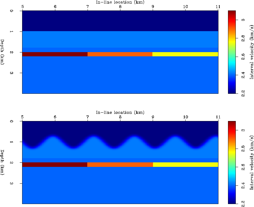
Figure 1 P-wave velocity models used to generate the synthetic data. Model 1 (top): overburden with flat layers, model 2 (bottom): overburden with velocity anomalies.
 |
In model 1, the overburden contains two flat layers with constant elastic properties on each layer, whereas model 2 includes a zone of complex velocity anomalies in the overburden. The rock properties for the model were taken from real well logs of a North Sea field. Typical values for different lithologies at this field are listed in Table 1.
| 1|c|Lithology | 1|c|Vp (km/s) | 1|c|Vs (km/s) | 1|c| |
| Shale | 2.4 | 0.95 | 2.25 |
| Cemented brine sands | 3.1 | 1.55 | 2.15 |
| Uncemented brine sands | 2.6 | 1.3 | 2.1 |
| Cemented oil sands | 2.9 | 1.6 | 2.05 |
| Uncemented oil sands | 2.35 | 1.33 | 2 |
| Volcanic ash (tuff) | 2.75 | 1.23 | 2.2 |
| Limestone | 4 | 2 | 2.4 |
Table 1. Typical rock properties for different lithologies at the North Sea.
Average values for overburden properties in the field are
Vp=2.2 km/s, Vs=0.75 km/s, ![]() (g/cm3).
(g/cm3).
In model 1, overburden properties above the flat
interface were taken to be the average values indicated above;
overburden properties
below the interface were the average values with a ![]() increase.
For model 2, we introduced lateral velocity anomalies
by including a smoothed sinusoidal interface between the two layers.
increase.
For model 2, we introduced lateral velocity anomalies
by including a smoothed sinusoidal interface between the two layers.