Velocity errors effect

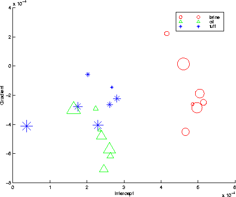
Using the synthetic data corresponding to model 2, we generated several migration-velocity realizations by introducing coherent percentage velocity errors at the overburden zone of the original velocity model. Using each velocity realization, we applied 2-D prestack wave-equation migration to the synthetic data; we applied an additional residual moveout correction and picked the resulting amplitudes. Figure 18 shows the crossplot of the intercept and gradient attributes at CIGs location which correspond to a valley of the sinusoidal irregularities; the size in the plot symbol increases as the velocity error increases. We can note that the intercept attribute is much less sensitive to velocity errors than the gradient attribute. 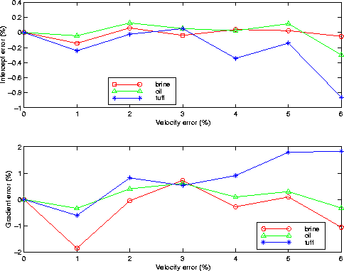Figure 19 shows the errors in the inverted attributes as a function of the velocity errors used in the migration. We can see that the maximum AVO intercept error is $34\%$ for velocity errors up to $5\%$ (tuff case), whereas for velocity errors of only 1%, the inversion of AVO gradient attribute (brine case) has an error of 185%.

 

mig_vel
Figure 18 Impact of velocity errors in Intercept versus Gradient crossplot

 

AB_error
Figure 19 Impact of velocity errors in Intercept and gradient attributes