next up previous print clean
Next: Missing data Up: Clapp: Regularizing with non-stationary Previous: Discontinuities and steering filters

Estimating a non-stationary filter

Another option is to characterize our model in terms of PEFs rather than steering filters. Normally we estimate a PEF by solving  
 \begin{displaymath}
\bold M \bold a \approx \bf 0
,\end{displaymath} (3)
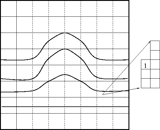
where $\bold M$ is convolution with a field that has the same properties as the model and $\bold a$ is our PEF. The output of this convolution is white Claerbout (1992a). Therefore $\bf a$ must have the inverse spectrum of the model. When the model varies continuously we must add a slight twist to our PEF estimation. Instead of breaking up our model space into regions where our stationary assumption is valid we are going to modify the PEF. Our PEF ($\bf a$) is now going to be composed of several different PEFs operating in micro-patches (Figure 9). With so many filters, and therefore filter coefficients, our filter estimation problem goes from being over-determined to under-determined. We can force the system to again be overdetermined by adding a regularization equation to our original filter estimation fitting goals,
\begin{eqnarray}
\bf 0&\approx&\bf M \bf a \\ \bf 0&\approx&\epsilon \bf F \bf a \nonumber \end{eqnarray} (4)
where the regularization operator $\bf F$ smoothes the filter coefficients Clapp et al. (1999).

 
patch
Figure 9
Non-stationary PEF construction. The model is broken up into micro-patches. Each micro-patch has its own PEF.
patch
view


next up previous print clean
Next: Missing data Up: Clapp: Regularizing with non-stationary Previous: Discontinuities and steering filters
Stanford Exploration Project
4/28/2000