|
bp-vel
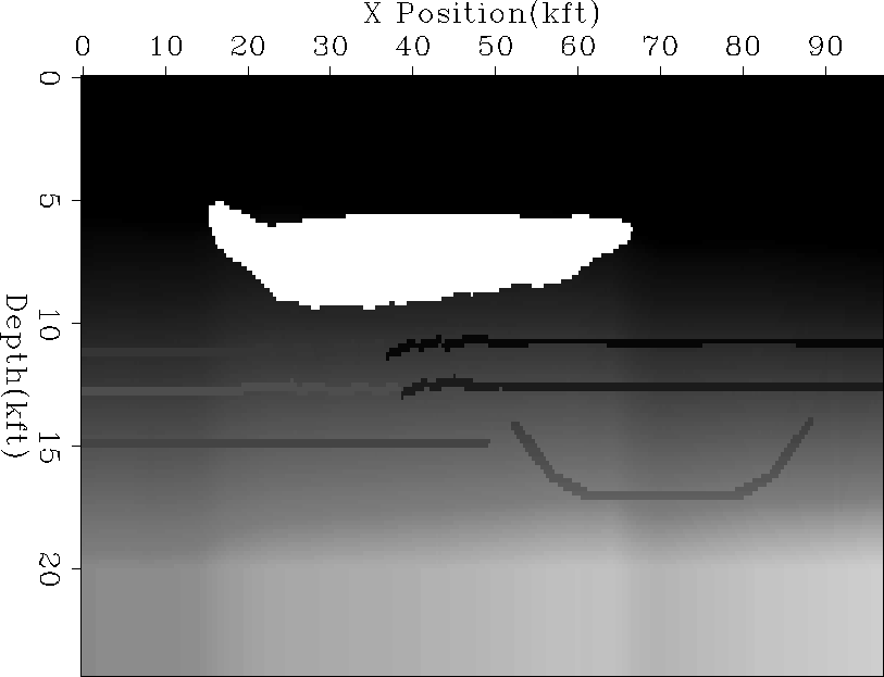
Figure 2 Synthetic velocity model for the BP dataset. |  |
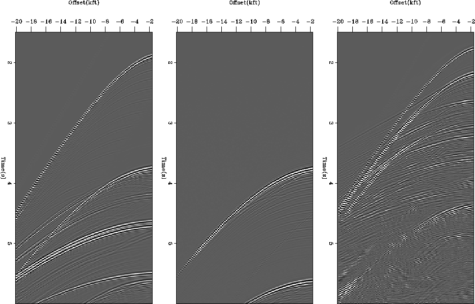
To test the method, we chose an elastic synthetic data generated by BP. Figure 2 is the p-wave velocity model used to construct the data. Within the model, multiple behavior ranged from rather simple (away from the salt body) to much more complex (along the edge and under the salt). We then modeled the multiples by doing frequency Kirchoff upward continuation of both the sources and receivers to the sea-floor. For our first test we chose a CMP gather at 1 kft, away from the salt edge. The left panel of Figure 3 shows the original CMP gather. The center panel shows the upward continued gather at the same location. The right panel shows the predicted signal for the CMP gather. Note that we have done a good job eliminating the multiples with little loss of primary energy.
|
bp-vel
Figure 2 Synthetic velocity model for the BP dataset. |  |
 |
Our second test was more of challenge. We chose a CMP through the salt at 44 kft (Figure 4). Note that both the primary and multiple energy is significantly more complicated than in the previous example. The right panel of Figure 4 again shows our primary estimate. In this case our primary estimate isn't quite as good as Figure 3 but we still have done an acceptable job reducing the multiple energy.
 |