Next: Convergence issues
Up: comparing IRLS and Huber
Previous: Tests on synthetic data:
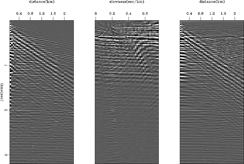
Figure 8 shows the input for the real data example. These data are contaminated with a
low velocity/low frequency noise crossing the main signal.
The Huber threshold and the damping paramater for IRLS are equal and obey the empirical choice
that we gave above. Figure 8 details the least-squares result. The
velocity panel (middle) shows some horizontal stripes that severely blur the main velocity fairway; in addition,
because no strong event appears below 1s., a poor resolution is achieved.
In regard to the l2 result, we might note that the remodeled data (right panel of Figure
8) exhibit some artifacts in the top part that shows
the limitations of the least-squares inversion in this case.
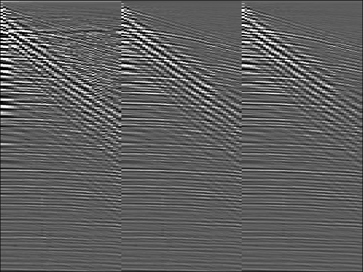
Figure 10 displays the ``l1'' inversion results with
the Huber solver and IRLS.
Again, because we are able to pick up a velocity fairway all the way down, both results are very comparable.
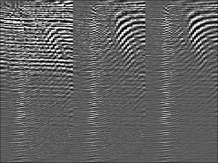
Moreover, the remodeled data (Figure 9) show fewer artifacts than they
do in the l2 case.
gr-wz08-L2-HUBER
Figure 8 From left to right: 1) Input data. 2) velocity
domain, l2 inversion result. 3) remodeled data from the l2 result


 comp-data-wz08-0.082
Figure 9 From left to right: 1) Remodeled data with l2.
2) Remodeled data with the Huber solver. 3) Remodeled data using IRLS
comp-mod-wz08-0.082
Figure 10 From left to right: 1) l2 velocity space.
2) Huber velocity space. 3) IRLS velocity space
Next: Convergence issues
Up: comparing IRLS and Huber
Previous: Tests on synthetic data:
Stanford Exploration Project
4/27/2000