Inversion results

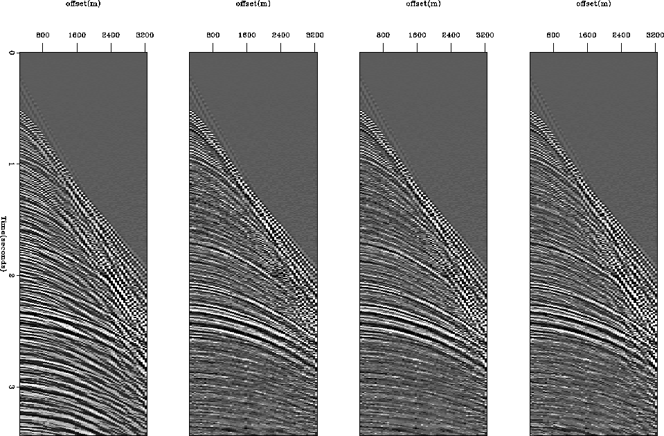
Figure 3 shows the result of the inversion for one CMP. Since the Mobil AVO dataset does not include very complex structures with strong velocity contrasts, this panel illustrates what happens for all the gathers. The left panel shows the input data. The other panels display the reconstructed data using the different schemes. Note that the l² and l¹ inversions give similar results and that the l¹ regularization doesn't converge as well. 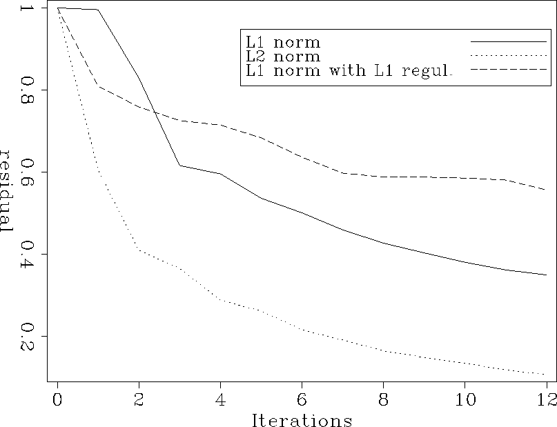Figure 4 highlights this difference between the different problems. The best convergence is achieved using least-squares and the worst is achieved with the l¹ regularization. 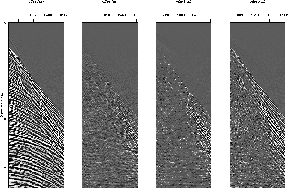In my implementation, however, the l¹ problem with or without regularization was solved using twice as many iterations as with l². Figure 5 shows the differences between the input data and the remodeled data. It appears that the l¹ norm with l¹ regularization encounters some difficulties in fitting the far offset data. Note that the l¹ norm and the l² norm are both comparable. This is expected since the data are not strongly noisy.

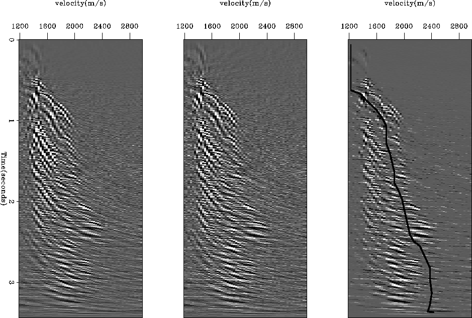
Differences arise in favor of the l¹ regularization when we look at the model space (Figure 6), however. The l¹ and l² results are again very similar and the l¹ norm with l¹ regularization appears spikier. This result is consistent with the theory (see Theory section). The spiky result is then used to define the limit between primaries and multiples (black line in the right panel of Figure 6). A mask is defined accordingly and the primaries are muted out in the model space. The next step consists of remodeling the multiples back in the data space, applying the hyperbola superposition principle (operator H). 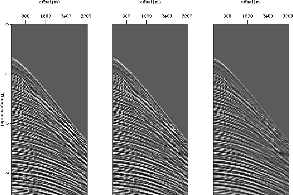Figure 7 shows the predicted multiples. Note that for the three inversion schemes, some primaries remain. This is particularly annoying to us in our attempt to produce true amplitude multiple-free gathers. Figure 8 displays the result of the multiple attenuation process. The three methods display similar results. Nonetheless, at far offset, the l¹ regularization shows more energetic events. This is consistent with Figure 5 where we showed that the l¹ regularization was unable to fit this part of the data.

 

comp_dat
Figure 3 Left: input data. Middle-left: l² reconstructed data. Middle-right: l¹ reconstructed data. Right: l¹ with l¹ regularization reconstructed data.

 

residual
Figure 4 Comparison of the convergence for different inversion schemes for one CMP gather.

 

diff
Figure 5 Left: input data. Middle-left: l² residual. Middle-right: l¹ residual. Right: l¹ with l¹ regularization residual.

 

comp_scan
Figure 6 Left:l² model. Middle: l¹ model. Right: l¹ with l¹ regularization. The line shows the limit of the muting process that separates ``guessed'' multiples on the left from ``guessed'' primaries on the right for the spiky model.

 

comp_mult
Figure 7 Predicted multiples. Left: l² multiples. Middle: l¹ multiples. Right: l¹ with l¹ regularization multiples.

 

comp
Figure 8 Gathers after multiple attenuation. Left: input data with multiples. Middle-left: l² multiple attenuation. Middle-right: l¹ multiple attenuation. Right: l¹ with l¹ regularization multiple attenuation.