|
102.smooth.out.closeup
Figure 9 Closeup of time-domain interpolation result using noise-free input. | 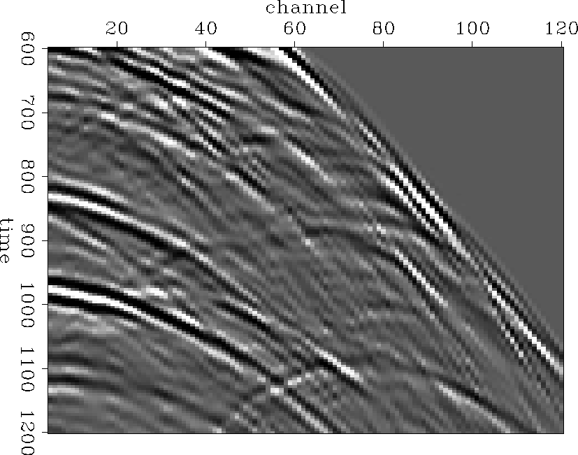 |
Interpolating in the frequency domain is generally faster than in the time domain, because convolution matrices turn diagonal and become multiplications. Normally, rather than bother with nonstationary convolution, the data are divided into patches and assumed to be locally stationary. As Margrave 1998 points out, Fourier transforms do not really imply stationarity, but nonstationary convolution in the time domain does not Fourier transform into a multiplication, but into a nonstationary combination, which is almost the same as a nonstationary convolution. It may turn out to be more or less expensive, depending on the number of nontrivial diagonals in the matrix, but it is not as quick as multiplication. With just enough effort to take out the obvious slack, I find that my own (t,x) interpolation takes several times longer than a canned commercial (f,x) interpolation (ProMAX), though that number varies significantly with parameterization, and might also vary a great deal with implementation. Unfortunately, I only had available an (f,x) version, and not (f,x,y). To be fair, the time-domain figures in this section are calculated using just t and x. Interpolation in (t,x,y) produces nicer figures, and presumably so does (f,x,y).
So why bother with the time domain? One answer is noise. Abma 1995 shows that (t,x) PEFs are less likely to create spurious events in the presence of noise, because calculating a filter at each frequency is the time domain equivalent of calculating a filter that is long on the time axis. The effective time length of the filter tends to give it sufficient freedom that it can predict the ostensibly random noise. On relatively noise-free data (such as the data in Figure 102.smooth.out), time- and frequency-domain implementations both produce good results. Closeups of a (t,x) and (f,x) interpolation result are shown in Figures 102.smooth.out.closeup and 102.smooth.fx.out.closeup. There are some examples of events that are better interpolated in the time domain, such as the event dipping steeply to the right in the very middle of closeups. However, it may be that someone with more experience at tuning the (f,x) parameter knobs would make that difference disappear. At any rate, either result is fine. With increasing amounts of noise, the time domain interpolation produces better results. Interpolated noisy gathers are shown in Figures 102.smooth.noise.out and 102.smooth.noise.fx.out. Noisy close ups are shown in Figures 102.smooth.noise.out.cp and 102.smooth.noise.fx.out.cp. Coherent noise, like multiples, will look just like signal and be interpolated right along with it. In the case of multiples, this is exactly the point of the interpolation. Interpolating the multiples dealiases them and makes them easier to suppress.
|
102.smooth.out.closeup
Figure 9 Closeup of time-domain interpolation result using noise-free input. |  |
|
102.smooth.fx.out.closeup
Figure 10 Closeup of frequency-domain interpolation result using noise-free input. | 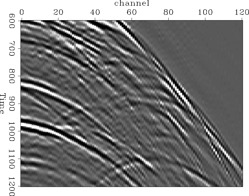 |
 |
 |
|
102.smooth.noise.out.cp
Figure 13 Closeup of time-domain interpolation result using noisy input. | 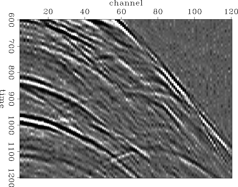 |
|
102.smooth.noise.fx.out.cp
Figure 14 Closeup of frequency-domain interpolation result using noisy input. | 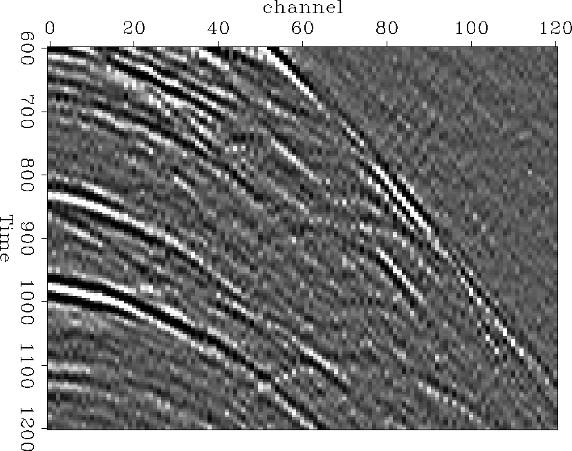 |