 |
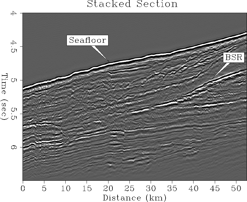
Figure 1 Christine Ecker's BSR data from her PhD disertation. Most reflectors are recognizeable as ``black-white-black''. The exception is the BSR reflector which is ``white-black-white''.
 |
In principle, a causal double integration converts this triplet into an impulse which theoretically should make for ready recognition of polarity. On the other hand, we need to think about whether the recording equipment actually records the low frequencies that double integration would amplify and we need to think about low-frequency noise.
 |
I have noticed
that marine recording systems often record seismic energy
right down to zero frequency.
This is evidenced by the appearance of water surface gravity waves
with speeds of about 30 km/hour,
speeds so slow that we can hardly distinguish their speed from zero.
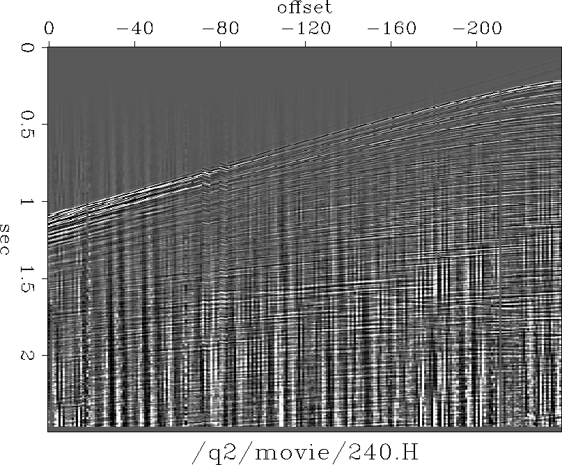
I have not made quantitative measurements on Figure 2,
but I believe it to be consistent with
long ocean swells moving about 20 miles/hour or 30 km/hour.
Distance traveled in meters over four seconds will be
![]() = 33m.
These become visible late on the data where the
t2 gain brings them up.
Their time signature is roughly a growing ramp function.
= 33m.
These become visible late on the data where the
t2 gain brings them up.
Their time signature is roughly a growing ramp function.
From these two data sets we recognize two different goals: One data set says we should use double integration to convert the (1,-2,1) ghost to a pulse. The other data set says we should use double differentiation to suppress the growing ramp function of the surface gravity waves.
On more careful study we can see that the goals
are not exactly opposite:
The ramp function rises over the full two seconds of the data.
Let us say its frequency is about .2 Hz.
On the other hand,
the triplet (1,-2,1)
is not merely spread over three samples but perhaps 10 samples or 40ms
so we associate it with a frequency of about 25 Hz.
Now imagine a data set with both the phenomena we see
on Figure 1 and
on Figure 2.
It would show both phenomena.
We can analyze this in the frequency domain or the time domain.
The composite spectrum would be the sum of their spectra.
The spectrum would grow near zero frequency as ![]() and grow near .2 Hz as
and grow near .2 Hz as ![]() .We need to raise the spectrum between those two limits
(or suppress it beyond those limits).
In the time domain we notice that
while the ramp function is approximately as long as the seismogram itself,
the duration of the triplet (1,-2,1) is about 10 samples or 40ms.
Perhaps the filter with the correct spectral characteristic
in the time domain would
begin as a ramp for 40ms
and then gently bend toward negative values a second or so later.
Notice that this is a fairly long filter
.We need to raise the spectrum between those two limits
(or suppress it beyond those limits).
In the time domain we notice that
while the ramp function is approximately as long as the seismogram itself,
the duration of the triplet (1,-2,1) is about 10 samples or 40ms.
Perhaps the filter with the correct spectral characteristic
in the time domain would
begin as a ramp for 40ms
and then gently bend toward negative values a second or so later.
Notice that this is a fairly long filter
We could examine the specifics more carefully but fortunately, the autoregression method of deconvolution addresses the general problem without requiring specific information. Notice a key ingredient here: The required autoregression filter, the PEF, is long because any approximation to double integration must be long. The filter length raises interesting issues that I have previously not given adequate attention to.
Basically we are talking about a decon filter whose length is a significant fraction of the trace length. There is a real danger that we might ``over fit'', i.e., use insufficient data to estimate the filter and find our filter adapting to the geology instead of adapting to the data-recording environment. The way to overcome this problem is to use a lot of data.