Forward operator: Perturbation migration

1.

Scattering and downward continuation

If we perturb the velocity model we introduce a perturbation in the wavefield. In other words, the perturbation in slowness generates a secondary wavefield, the scattered wavefield. We can downward continue the scattered field as we did with the background wavefield by writing  

$$\fbox {$ \Delta u^{z+1}(\omega_{\!}) = T_0^{z}(\omega_{\!},s_0) \Delta u^{z}(\omega_{\!}) + \Delta v^{z+1}(\omega_{\!}) $}$$ (20)

where

• $\Delta u^{z}(\omega_{\!})$ is the perturbation in the wavefield generated by the perturbation in velocity, and
• $\Delta v^{z+1}(\omega_{\!})$ represents the scattered wavefield caused at depth level z+1 by the perturbation in velocity from the depth level z.

The scattered wavefield can be written as  

$$\Delta v^{z+1}(\omega_{\!}) = T_0^{z}(\omega_{\!},s_0) G_0^{z}(\omega_{\!},s_0) u_0^{z}(\omega_{\!}) \Delta s^{z}(\omega_{\!})$$ (21)

where

• $G_0^{z}(\omega_{\!},s_0)$ is the scattering operator at depth z, and
• $\Delta s^{z}(\omega_{\!})$ is the perturbation in slowness at depth z.

Huang et al. 1999 show that the scattering operator is

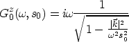$$G_0^{z}(\omega_{\!},s_0) = i\omega_{\!} \frac{1}{\sqrt{1-\frac{\vert\vec{k}\vert^2}{\omega_{\!}^2s_0^2}}}$$ (22)

and that it can be approximated by

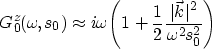$$G_0^{z}(\omega_{\!},s_0) \approx i\omega_{\!} \left(1+\frac{1}{2}\frac{\vert\vec{k}\vert^2}{\omega_{\!}^2s_0^2}\right)$$ (23)

which represents the first-order Born approximation. In this equation, $\vec{k}$ represents the horizontal component of the wavenumber.

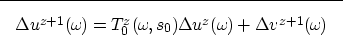
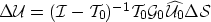
If we introduce Equation (B-2) into (B-1) we obtain

$$\Delta u^{z+1} = T_0^{z} \left[ \Delta u^{z} + G_0^{z} u_0^{z} \Delta s^{z} \right]$$ (24)

which, after rearrangements, becomes the recursion  

$$\Delta u^{z+1} - T_0^{z} \Delta u^{z} = T_0^{z} G_0^{z} u_0^{z} \Delta s^{z}$$ (25)

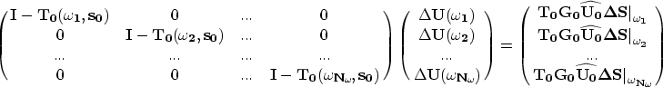
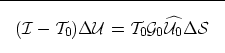
We can express the recursive relationship between the perturbation in velocity and the perturbation in the wavefield (B-6) as  

$$\fbox {$ [\bf {I}-\bf {T_0}]\Delta \bf{U}= \bf {T_0}\bf {G_0}\widehat {\bf{U_0}}\Delta \bf{\S}$}$$ (26)

$$\begin{eqnarray} \left[ \matrix { {1} & 0 & 0 &...& 0 & 0 \cr {-T_0^{1}} & {1} &... ...2}\cr \Delta s^{3}\cr...\cr \Delta s^{N_z} \cr } \right]\nonumber \end{eqnarray}$$

where

• $\Delta \bf{U}$ is a column vector containing the perturbation in the wavefield at all depths,
• $\bf {G_0}$ is a diagonal matrix containing the scattering term for all the depth levels,
• $\widehat {\bf{U_0}}$ is a diagonal matrix containing the background wavefield data for all the depth levels, and
• $\Delta \bf{\S}$ is a column vector containing the perturbation in the velocity for all the depth levels.

Note the different arrangement of the background wavefield data at all depths ($\bf{U_0}$ and $\widehat {\bf{U_0}}$).

Similarly to the case of the background wavefield, the relationship between the perturbation in the wavefield and the perturbation in slowness can be written for all the frequencies in the data as

$$\fbox {$ (\mathcal I-\mathcal T_0) \Delta \mathcal U= \mathcal T_0\mathcal G_0\widehat{\mathcal U_0}\Delta \mathcal \S $}$$ (27)

$$\begin{eqnarray} \left( \matrix { {\bf {I}-\bf {T_0}{(\omega_{1},s_0)}} & 0 &...... ...bf{\S}\big\vert _{\omega_{N_{\omega_{\!}}}}\cr } \right)\nonumber \end{eqnarray}$$

where

• $\Delta \mathcal U$ is a column vector containing the perturbation in the wavefield for all the frequencies,
• $\mathcal G_0$ is a diagonal matrix containing the scattering operator for all the frequencies,
• $\widehat{\mathcal U_0}$ is a diagonal matrix containing the background wavefield for all the frequencies, and
• $\Delta \mathcal \S$ is a column vector containing the perturbation in slowness, same for all the frequencies if we disregard dispersion.

Again, it is important to note the different arrangement of the background wavefield data at all frequencies ($\mathcal U_0$ and $\widehat{\mathcal U_0}$).

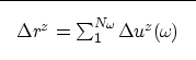
Therefore, we can compute the perturbation in the wavefield ($\Delta \mathcal U$) as a function of the perturbation in slowness ($\Delta \mathcal \S$) like this:

$$\Delta \mathcal U= (\mathcal I-\mathcal T_0)^{-1} \mathcal T_0\mathcal G_0\widehat{\mathcal U_0}\Delta \mathcal \S$$ (28)

2.

Imaging

As for the background image, the perturbation in image ($\Delta \i^{z}$), caused by the perturbation in slowness, is obtained by a summation over all the frequencies ($\omega_{\!}$):  

$$\fbox {$ \Delta \i^{z} = \sum_1^{N_{\omega_{\!}}} \Delta u^{z}(\omega_{\!}) $}$$ (29)

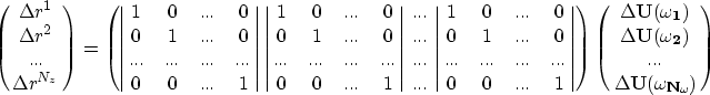
We can write Equation (B-10) in matrix form as  

$$\fbox {$ \Delta \mathcal R= \mathcal H\Delta \mathcal U $}$$ (30)

$$\begin{eqnarray} \left( \matrix{ \Delta \i^{1} \cr \Delta \i^{2} \cr ...\cr \Del... ... \Delta \bf{U}{(\omega_{N_{\omega_{\!}}})} \cr } \right)\nonumber \end{eqnarray}$$

where

• $\Delta \mathcal R$ is a column vector containing the perturbation in image at every depth level z.

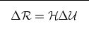
Therefore, the perturbation in image ($\Delta \mathcal R$), corresponding to the perturbation velocity field ($\Delta \mathcal \S$), can be computed as follows:  

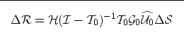$$\fbox {$ \Delta \mathcal R= \mathcal H(\mathcal I-\mathcal ... ...al T_0\mathcal G_0\widehat{\mathcal U_0}\Delta \mathcal \S $}$$ (31)