


Next: Noise Free Data
Up: Symes: Differential semblance
Previous: Admissible Models
The convolutional offset trace model is one of those for which the forward
modeling operator on a minimal gather, ie. a single
trace, is invertible. The inverse operator is
![\begin{displaymath}
G[v]S(t_0,x)=\frac{S(T(t_0,x),x)}{a(T(t_0,x),x)}\end{displaymath}](img20.gif)
The operator measuring semblance differentially is

Then
![\begin{displaymath}
F[v]WG[v]S(t,x)=a(t,x)\left[\frac{\partial}{\partial x}
\frac{S(T(t_0,x),x)}{a(T(t_0,x),x)}\right]_{t_0=T_0(t,x)}\end{displaymath}](img22.gif)
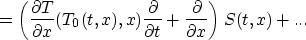
where
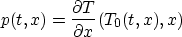
is the arrival (horizontal) slowness of the ray passing offset x at time
t, and the elided terms involve the amplitude a, but do not involve
derivatives of the data S. Thus these terms are of lower frequency content
than the leading term (explicitly displayed), and are of the same relative
order in frequency as terms neglected in the derivation of the convolutional
model from the acoustic wave equation. Therefore they can be dropped: this
leads to the remarkable conclusion that the differential semblance objective
is independent of the amplitude at least to leading order in frequency.
This observation is due to Hua Song. As a result, within accuracy
limitations already built into the asymptotic linearized model, a
might as well be replaced by 1!. That is, to leading order in
frequency, differential semblance is insensitive to wave dynamics
(amplitude), and responds only to kinematic model changes,
i.e. changes in traveltime. Thus minimization of differential
semblance will amount to a sort of traveltime tomography.
Fons ten Kroode (personal communication) has pointed out that
replacement of G[v] by an asymptotically unitary operator with
the same kinematics also yields an asymptotocally identical
objective without leading order amplitude dependence, and without
application of the forward modeling operator, thus at lower computational
cost.
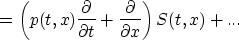
The computations above are correct when the map  is smooth and invertible. This is so inside the mute zone
defined above, uniformly for
is smooth and invertible. This is so inside the mute zone
defined above, uniformly for  . Therefore application of
the inverse square root Helmholtz operator following will bring the
spectral content back into alignment with that of the data, uniformly
over . Thus
. Therefore application of
the inverse square root Helmholtz operator following will bring the
spectral content back into alignment with that of the data, uniformly
over . Thus
![\begin{displaymath}
H \phi F[v]WG[v]S = H \phi \left(\frac{\partial S}{\partial x}+p
\frac{\partial S}{\partial t}\right) + O(\lambda)\end{displaymath}](img28.gif)
The ray slowness p is locally a smooth function of the velocity v
in any fixed open subset of the mute zone, hence J0 (which is the
mean square of the above expression) is a smooth function of as well.
Next: Noise Free Data
Up: Symes: Differential semblance
Previous: Admissible Models
Stanford Exploration Project
4/20/1999