|
data
Figure 4 The input data are irregularly sampled. |  |
|
data
Figure 4 The input data are irregularly sampled. |  |
The first example is a simple synthetic test for 1-D inverse
interpolation. The input data were randomly subsampled (with
decreasing density) from a sinusoid (Figure 4). The
forward operator ![]() in this case is linear interpolation. We seek
a regularly sampled model that could predict the data with a
forward linear interpolation. Sparse irregular distribution of the
input data makes the regularization enforcement a necessity.
I applied convolution with the simple (1,-1)
difference filter as the operator
in this case is linear interpolation. We seek
a regularly sampled model that could predict the data with a
forward linear interpolation. Sparse irregular distribution of the
input data makes the regularization enforcement a necessity.
I applied convolution with the simple (1,-1)
difference filter as the operator ![]() that forces model continuity
(the first-order spline).
An appropriate preconditioner
that forces model continuity
(the first-order spline).
An appropriate preconditioner ![]() in this
case is recursive causal integration.
in this
case is recursive causal integration.
 |
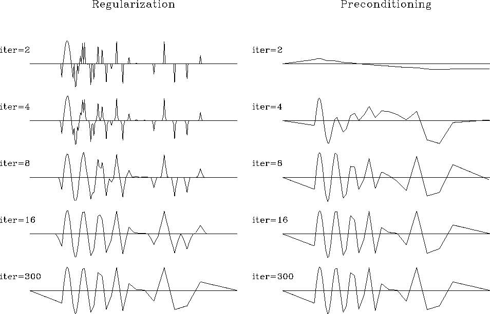
As expected, preconditioning provides a much faster rate of convergence. Since iteration to the exact solution is never achieved in large-scale problems, the results of iterative optimization may turn out quite differently. Bill Harlan points out that the two components of the model-space regularization [equations (8) and (8)] conflict with each other: the first one enforces ``details'' in the model, while the second one tries to smooth them out. Typically, regularized optimization creates a complicated model at early iterations. At first, the data fitting goal (8) plays a more important role. Later, the regularization goal (8) comes into play and simplifies (smooths) the model as much as needed. Preconditioning acts differently. The very first iterations create a simplified (smooth) model. Later, the data fitting goal adds more details into the model. If we stop the iterative process early, we end up with an insufficiently complex model, not in an insufficiently simplified one. Figure 5 provides a clear illustration of Harlan's observation.
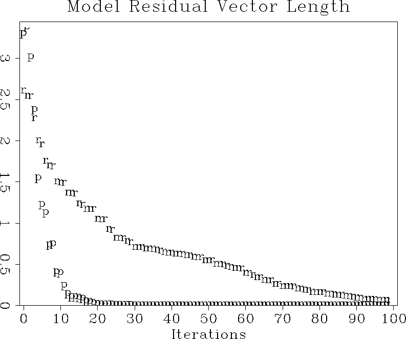
Following Matthias Schwab's suggestion, I measured the rate of convergence by the model residual, which is a distance from the current model to the final solution. Figure 6 shows that the data regularization method converged to the final solution in many fewer iterations than the model regularization. Since the cost of each iteration for each method is roughly equal, the efficiency of preconditioning is evident. Figure 5 shows the final solution, and the estimates from preconditioning and regularization after different numbers of conjugate-direction iterations. At early iterations, the preconditioning estimate is much closer to the final solution.
|
schwab1
Figure 6 Convergence of the iterative optimization, measured in terms of the model residual. The ``p'' points stand for preconditioning; the ``r'' points, regularization. |  |
module invint2 {   # Inverse linear interpolation
  use lint1
  use helicon      # regularized    by helix   filtering
  use polydiv      # preconditioned by inverse filtering
  use cgstep_mod
  use solver_mod
contains
  subroutine invint1( niter, coord, ord, o1,d1, mm,mmov, eps, aa,lag, precon) {
    logical,                  intent( in)  :: precon
    integer,                  intent( in)  :: niter
    real,                     intent( in)  :: o1, d1, eps
    real,    dimension( :),   intent( in)  :: ord
    real,    dimension( :),   intent( out) :: mm
    real,    dimension( :,:), intent( out) :: mmov         # model movie
    real,    dimension( :),   pointer      :: coord, aa    # coordinate, filter
    integer, dimension( :),   pointer      :: lag          # filter lag
    call lint1_init( o1, d1, coord)
    if( precon) {                                          # preconditioning
       call polydiv_init( aa, lag)
       call solver_prec( lint1_lop, cgstep, niter = niter, x = mm, dat = ord,
                    prec = polydiv_lop, nprec = size(mm), eps = eps,
                    xmov = mmov)
    } else {                                               # regularization
       call helicon_init( aa, lag)
       call solver_reg(  lint1_lop, cgstep, niter = niter, x = mm, dat = ord,
                    reg = helicon_lop, nreg = size(mm), eps = eps,
                    xmov = mmov)
    }
    call cgstep_close()
  }
}