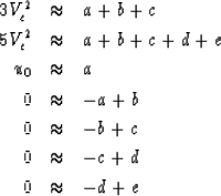
Sometimes we seek a velocity model that increases smoothly with depth through our scattered measurements of good-quality RMS velocities. Other times, we seek a blocky model. (Where seismic data is poor, a well log could tell us whether to choose smooth or blocky.) Here we see an estimation method that can choose the blocky alternative, or some combination of smooth and blocky.
Consider a five layer model, each layer having unit traveltime thickness (so integration is simply summation). Let the squared interval velocities be (a,b,c,d,e) with strong reliable reflections at the base of layer c and layer e, and weak, incoherent, ``bad'' reflections at bases of (a,b,d). Thus we measure Vc2 the RMS velocity squared of the top three layers and Vd2 that for all five layers. Since we have no reflection from at the base of the fourth layer, the velocity in the fourth layer is not measured but a matter for choice. In a smooth linear fit we would want d=(c+e)/2. In a blocky fit we would want d=e.
Our screen for good reflections looks like (0,0,1,0,1)
and our screen for bad ones looks like the complement (1,1,0,1,0).
We put these screens on the diagonals of diagonal matrices
![]() and
and ![]() .Our fitting goals are:
.Our fitting goals are:
 |
(15) | |
| (16) | ||
| (17) | ||
| (18) | ||
| (19) | ||
| (20) | ||
| (21) |
| (22) | ||
| (23) |
| |
(24) |
| |
(25) |
The formulation
(25)
is so logical that we might have guessed it:
The goal ![]() says that
says that ![]() is mostly zero.
What emerges from
is mostly zero.
What emerges from ![]() is a sprinkling of impulses.
Then
is a sprinkling of impulses.
Then ![]() converts the pulses to ramp functions
(zero until a certain place, then growing linearly)
which are used to fit the data (integrated velocity).
Differentiating the data-fitting ramps
converts them to the desired blocks of constant velocity.
One iteration is required for each impulse.
converts the pulses to ramp functions
(zero until a certain place, then growing linearly)
which are used to fit the data (integrated velocity).
Differentiating the data-fitting ramps
converts them to the desired blocks of constant velocity.
One iteration is required for each impulse.
Choosing ![]() to be an identity
to be an identity ![]() gives smooth velocity models,
such as caused by the increasing consolidation of the rocks with depth.
Choosing the screen
gives smooth velocity models,
such as caused by the increasing consolidation of the rocks with depth.
Choosing the screen ![]() to have a sprinkling of pass locations
picks the boundaries of blocks of constant velocity.
The choice can be made by people with subjective criteria (like geologists)
or we can assist by using the data itself
in various ways to select our degree of preference between
the blocky and smooth models.
For example,
we could put seismic coherency or amplitude
on the goodpass diagonal matrix
to have a sprinkling of pass locations
picks the boundaries of blocks of constant velocity.
The choice can be made by people with subjective criteria (like geologists)
or we can assist by using the data itself
in various ways to select our degree of preference between
the blocky and smooth models.
For example,
we could put seismic coherency or amplitude
on the goodpass diagonal matrix ![]() .Clearly, much remains to be gained from experience.
.Clearly, much remains to be gained from experience.