![\begin{displaymath}
\bold 0
\quad \approx \quad
\bold r \eq
\left[
\begin{array...
..._2 \\
y_3 \\
y_4 \\
y_5 \\
y_6 \end{array} \right] \end{displaymath}](img21.gif)
![\begin{displaymath}
\bold 0
\quad \approx \quad
\bold r \eq
\left[
\begin{array...
..._2 \\
y_3 \\
y_4 \\
y_5 \\
y_6 \end{array} \right] \end{displaymath}](img21.gif) |
(9) |
![\begin{displaymath}
\left[
\begin{array}
{c}
0 \\
0 \\
0 \\
0 \\
0...
...
\begin{array}
{c}
1 \\
-f_1 \\
-f_2 \end{array} \right]\end{displaymath}](img23.gif) |
(10) |
Multiple reflections are predictable. It is the unpredictable part of a signal, the prediction residual, that contains the primary information. The output of the filter (1,-f1, -f2) = (a0, a1, a2) is the unpredictable part of the input. This filter is a simple example of a ``prediction-error'' (PE) filter.
It is one member of a family of filters called ``error filters.''
The error-filter family are filters with one coefficient constrained to be unity and various other coefficients constrained to be zero. Otherwise, the filter coefficients are chosen to have minimum power output. Names for various error filters follow:
 prediction-error (PE) filter
		gapped PE filter with a gap
 interpolation-error (IE) filter
We introduce a
free-mask matrix ![]() which ``passes'' the freely variable coefficients in the filter
and ``rejects'' the constrained coefficients
(which in this first example is merely the first coefficient a0=1).
which ``passes'' the freely variable coefficients in the filter
and ``rejects'' the constrained coefficients
(which in this first example is merely the first coefficient a0=1).
![\begin{displaymath}
\bold K \eq
\left[
\begin{array}
{cccccc}
0 & . & . \\ . & 1 & . \\ . & . & 1
\end{array} \right]\end{displaymath}](img28.gif) |
(11) |
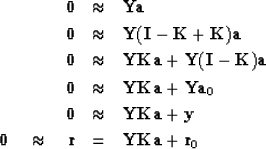
To compute a simple prediction error filter ![]() with the CD method,
we write
(9) or
(10) as
with the CD method,
we write
(9) or
(10) as
![\begin{displaymath}
\bold 0
\quad \approx \quad
\bold r \eq
\left[
\begin{array...
..._2 \\
y_3 \\
y_4 \\
y_5 \\
y_6 \end{array} \right] \end{displaymath}](img30.gif) |
(12) |
![[*]](http://sepwww.stanford.edu/latex2html/cross_ref_motif.gif) ).)
The fitting goal is,
).)
The fitting goal is,
 |
(13) | |
| (14) | ||
| (15) | ||
| (16) | ||
| (17) | ||
| (18) |
| (19) | ||
| (20) |
module gdecon_mod { # gapped deconvolution.  input=yy  output=rr
  use icaf1
  use cgstep_mod
  use solver_mod
contains
  subroutine gdecon( na, yy, rr, niter, gap) {
    integer,                intent( in)  :: na, niter, gap
    real,    dimension( :), pointer      :: yy
    real,    dimension( :), intent( out) :: rr
    real,    dimension( na)              :: aa # prediction-error filter
    logical, dimension( na)              :: mm # filter mask
    real,    dimension( size( yy))       :: dd # data
    dd = 0.                                    # initialize data
    aa = 0.; aa( 1) = 1.                       # initialize filter
    mm = .false.; mm( :gap) = .true.           # initialize mask
    call icaf1_init( yy, 1)                    # initialize convolution
    call solver( icaf1_lop, cgstep, aa, dd, niter,
                 x0= aa, res= rr, known= mm)
    call cgstep_close()
  }
}
My previous book, PVI, has many examples of gapped deconvolution on real and synthetic data. This book develops more two-dimensional examples.