|
rabdomain
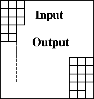
Figure 5 Domain of inputs and outputs of a two-dimensional filter like a PEF. |  |
Sometimes we deal with small patches of data. In order that boundary phenomena not dominate the calculation intended in the central region, we need to take care that input data is not assumed to be zero beyond the interval that the data is given. Examine figure 5
|
rabdomain
Figure 5 Domain of inputs and outputs of a two-dimensional filter like a PEF. |  |
There are two things to understand about Fig 5.
First, keeping the filter inside the outer box,
we get outputs only in the inner box.
Second, (the adjoint idea) crosscorrelating the inner and outer boxes gives
us the ![]() patch of information
we use to build the filter coefficients.
We need to be careful not to assume
that signals vanish outside the region where they are defined.
In a later chapter we will break data spaces into overlapping segments,
separately analyze the patches, and put everything back together.
We do this because crosscorrelations change with time
and they are handled as constant in short time windows.
There we must be particularly careful that zero signal values not be presumed
off the ends of the small volumes;
otherwise the many edges and faces of the many small volumes
can overwhelm the interior that we want to study.
patch of information
we use to build the filter coefficients.
We need to be careful not to assume
that signals vanish outside the region where they are defined.
In a later chapter we will break data spaces into overlapping segments,
separately analyze the patches, and put everything back together.
We do this because crosscorrelations change with time
and they are handled as constant in short time windows.
There we must be particularly careful that zero signal values not be presumed
off the ends of the small volumes;
otherwise the many edges and faces of the many small volumes
can overwhelm the interior that we want to study.
In practice, the input and output are allocated equal memory, but the output residual is initialized to zero everywhere and then not computed except where shown in figure 5. Below is Sergey Fomel's module boundary to build a selector for filter outputs that should be empty. There are two regions to think about: (1) at the beginning where the filter is moving onto the helix, (the left side in Fig 5). and (2) on the ``backside'' of the helix (top and bottom in Fig 5) where the filter moves off of one loop and onto the next. With Fig 5, you should be able to understand the two-dimensional parts of the the module boundary. (The 3-D part will test your visualization skills.)
module boundary {     # mark helix filter outputs where input is off data.
contains
  subroutine bound3 (n1, n2, lag1, lag2, a1, a2, a3, misin) {
    integer, intent (in)   :: a1, a2, a3, n1, n2, lag1, lag2
    logical, dimension (:) :: misin
    integer                :: i1, i2, i, n123
    n123 = size( misin)
    misin = .false.
			    # This is the transient onset onto the helix
    do i=1, a1-1        { misin(i)=.true.}    # 1-D
    do i=1,(a2-1)*n1    { misin(i)=.true.}    # 2-D
    do i=1,(a3-1)*n1*n2 { misin(i)=.true.}    # 3-D
			    # These disconnect each loop from the next.
    do i1 = 1, lag1-1       { do i =    i1, n123,    n1 { misin(i) = .true.}}
    do i1 = n1-a1+lag1+1,n1 { do i =    i1, n123,    n1 { misin(i) = .true.}}
    do i2 = 1, lag2-1       { do i = i2*n1, n123, n2*n1 { misin(i) = .true.}}
    do i2 = n2-a2+lag2+1,n2 { do i = i2*n1, n123, n2*n1 { misin(i) = .true.}}
  }
}