MISSING DATA IN ONE DIMENSION

A method for restoring missing data is to ensure that the restored data, after specified filtering, has minimum energy. Specifying the filter chooses the interpolation philosophy. Generally the filter is a roughening filter.

When a roughening filter goes off the end of smooth data, it typically produces a big end transient. Minimizing energy implies a choice for unknown data values at the end, to minimize the transient. We will examine five cases and then make some generalizations.

A method for restoring missing data is to ensure that the restored data, after specified filtering, has minimum energy.

Let u denote an unknown (missing) value. The dataset on which the examples are based is $(\cdots, u, u,$ $1, u, 2, 1, 2, u, u, \cdots )$.Theoretically we could adjust the missing u values (each different) to minimize the energy in the unfiltered data. Those adjusted values would obviously turn out to be all zeros. The unfiltered data is data that has been filtered by an impulse function. To find the missing values that minimize energy out of other filters, we can use subroutine mis1() . Figure 1 shows interpolation of the dataset with (1,-1) as a roughening filter. The interpolated data matches the given data where they overlap.

 

mlines90 Figure 1 Top is given data. Middle is given data with interpolated values. Missing values seem to be interpolated by straight lines. Bottom shows the filter (1,-1), whose output has minimum energy.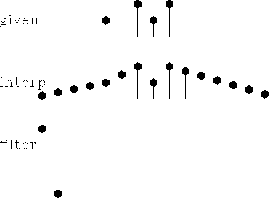

 

mparab90 Figure 2 Top is the same input data as in Figure 1. Middle is interpolated. Bottom shows the filter (-1,2,-1). The missing data seems to be interpolated by parabolas.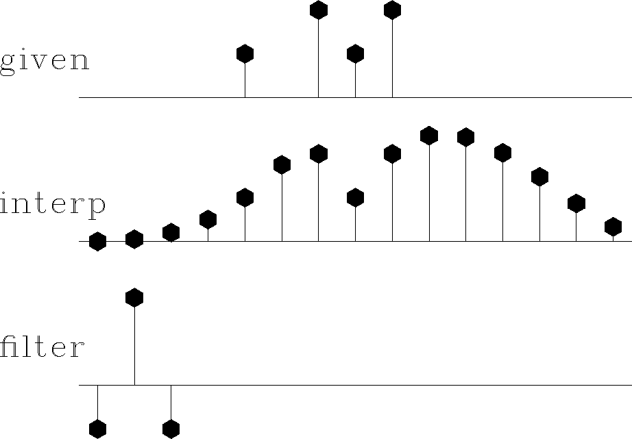

 

mseis90 Figure 3 Top is the same input. Middle is interpolated. Bottom shows the filter (1,-3,3,-1). The missing data is very smooth. It shoots upward high off the right end of the observations, apparently to match the data slope there.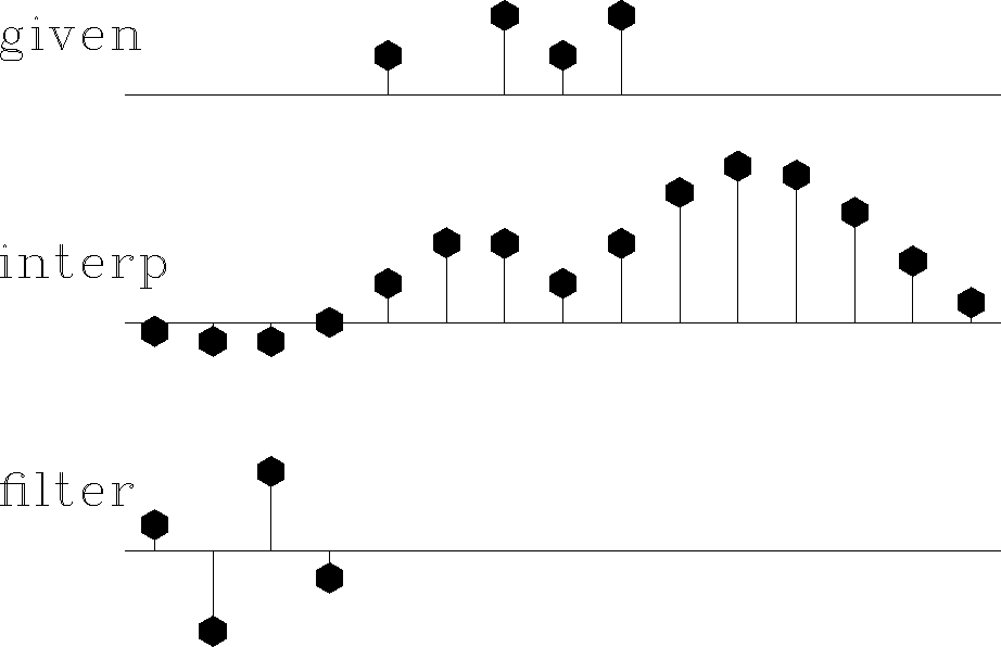

 

moscil90 Figure 4 Bottom shows the filter (1,1). The interpolation is rough. Like the given data itself, the interpolation has much energy at the Nyquist frequency. But unlike the given data, it has little zero-frequency energy.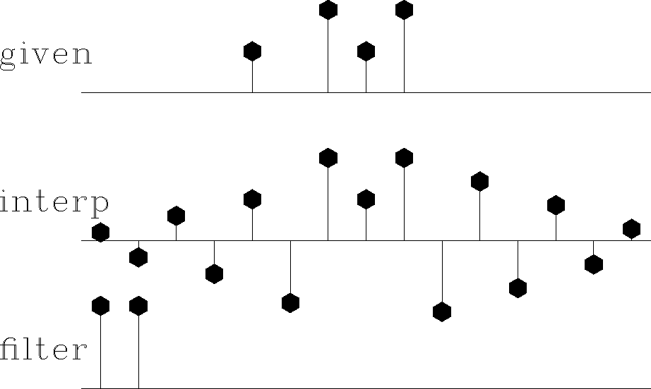

Figures 1-4 illustrate that the rougher the filter, the smoother the interpolated data, and vice versa. Let us switch our attention from the residual spectrum to the residual itself. The residual for Figure 1 is the slope of the signal (because the filter (1,-1) is a first derivative), and the slope is constant (uniformly distributed) along the straight lines where the least-squares procedure is choosing signal values. So these examples confirm the idea that the least-squares method abhors large values (because they are squared). Thus, least squares tends to distribute residuals uniformly in both time and frequency to the extent allowed by the constraints.

This idea helps us answer the question, what is the best filter to use? It suggests choosing the filter to have an amplitude spectrum that is inverse to the spectrum we want for the interpolated data. A systematic approach is given in chapter , but I offer a simple subjective analysis here: Looking at the data, we see that all points are positive. It seems, therefore, that the data is rich in low frequencies; thus the filter should contain something like (1,-1), which vanishes at zero frequency. Likewise, the data seems to contain Nyquist frequency, so the filter should contain (1,1). The result of using the filter $(1,-1)\ast (1,1)=(1,0,-1)$is shown in Figure 5. This is my best subjective interpolation based on the idea that the missing data should look like the given data. The interpolation and extrapolations are so good that you can hardly guess which data values are given and which are interpolated.

 

mbest90 Figure 5 Top is the same as in Figures 1 to 4. Middle is interpolated. Bottom shows the filter (1,0,-1), which comes from the coefficients of 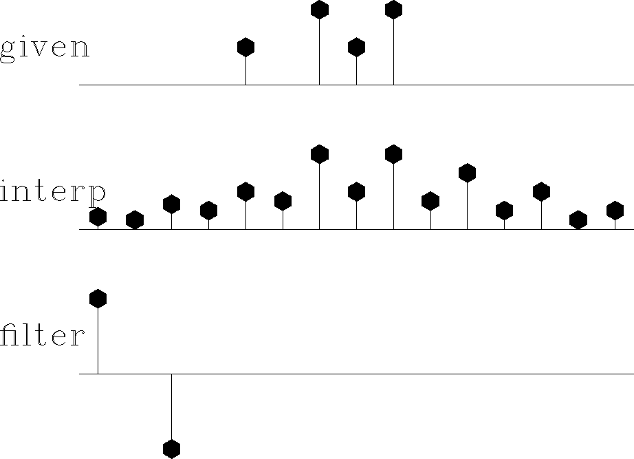$(1,-1)\ast (1,1)$. Both the given data and the interpolated data have significant energy at both zero and Nyquist frequencies.