 |
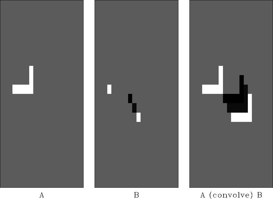
Figure 1 Two-dimensional convolution (as performed in one dimension).
 |
A surprising, indeed amazing, fact is that Figure 1 was not computed with a two-dimensional convolution program. It was computed with a one-dimensional computer program. It could have been done with anybody's one-dimensional convolution program, either in the time domain or in the fourier domain. This magical trick is done with the helical coordinate system.
A basic idea of filtering, be it in one dimension, two dimensions, or more, is that you have some filter coefficients and some sampled data; you pass the filter over the data; at each location you find an output by crossmultiplying the filter coefficients times the underlying data and summing the terms.
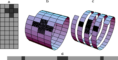
The helical coordinate system is much simpler than you might imagine. Ordinarily, a plane of data is thought of as a collection of columns, side by side. Instead, imagine the columns stored end-to-end, and then coiled around a cylinder. This is the helix. Fortran programmers will recognize that Fortran's way of storing 2-D arrays in one-dimensional memory is exactly what we need for this helical mapping. Seismologists sometimes use the word ``supertrace'' to describe a collection of seismograms stored ``end-to-end''.
Figure 2 shows a helical mesh for 2-D data on a cylinder. Darkened squares depict a 2-D filter shaped like the Laplacian operator. The input data, the filter, and the output data are all on helical meshes all of which could be unrolled into linear strips. A compact 2-D filter like a Laplacian, on a helix is a sparse 1-D filter with long empty gaps.
 |
Since the values output from filtering can be computed in any order, we can slide the filter coil over the data coil in any direction. The order that you produce the outputs is irrelevant. You could compute the results in parallel. We could, however, slide the filter over the data in the screwing order that a nut passes over a bolt. The screw order is the same order that would be used if we were to unwind the coils into one-dimensional strips and convolve them across one another. The same filter coefficients overlay the same data values if the 2-D coils are unwound into 1-D strips. The helix idea allows us to obtain the same convolution output in either of two ways, a one-dimensional way, or a two-dimensional way. I used the one-dimensional way to compute the obviously two-dimensional result in Figure 1.
Deconvolution (polynomial division) can undo convolution (polynomial multiplication). A magical property of the helix is that we can consider 1-D convolution to be the same as 2-D convolution. Hence is a second magical property: We can use 1-D deconvolution to undo convolution, whether that convolution was 1-D or 2-D. Thus, we have discovered how to undo 2-D convolution. We have discovered that 2-D deconvolution on a helix is equivalent to 1-D deconvolution. The helix enables us to do multidimensional deconvolution.
Deconvolution is recursive filtering. Recursive filter outputs cannot be computed in parallel, but must be computed sequentially as in one dimension, namely, in the order that the nut screws on the bolt.
Recursive filtering sometimes solves big problems with astonishing speed. It can propagate energy rapidly for long distances. Unfortunately, recursive filtering can also be unstable. The most interesting case, near resonance, is also near instability. There is a large literature and extensive technology about recursive filtering in one dimension. The helix allows us to apply that technology to two (and more) dimensions. It is a huge technological breakthrough.
In 3-D we simply append one plane after another (like a 3-D Fortran array). It is easier to code than to explain or visualize a spool or torus wrapped with string, etc.