PEFs on both model space and residual space

Finally, let us use PEFs in both data space and map space.  

$$\begin{array} {lll} 0 &\approx & \bold W \bold A ( \bold B ... ... \bold h \\ 0 &\approx & \epsilon \bold V \bold h \end{array}$$ (8)

I omit the display of my subroutine for the goals (8) because the code is so similar to potato(). (Its name is pear() and it is in the library.)

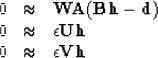
A disadvantage of the previous result in Figure 7 is that for the horizontal gradient, the figure is dark on one side and light on the other, and likewise for the vertical gradient. Looking at the result in Figure 8 we see that this is no longer true. Thus although the topographic PEFs look similar to a gradient, the difference is substantial.

 

pear
Figure 8 Galilee residuals estimated by (8).

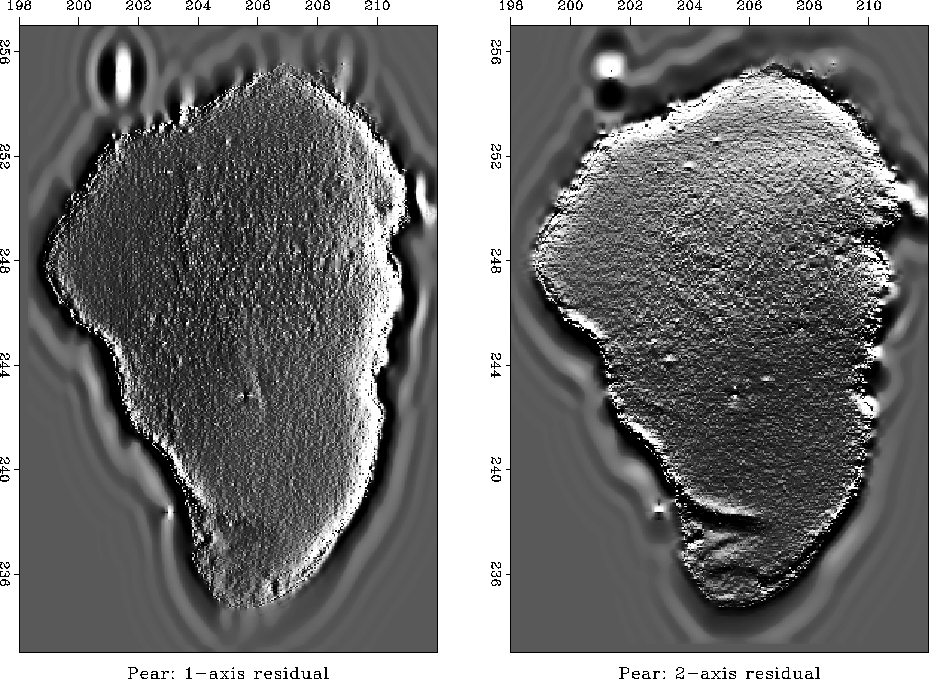Subjectively comparing Figures 7 and 8 our preference depends partly on what we are looking at and partly on whether we view the maps on paper or a computer screen. Having worked on this so long, I am disappointed that most of my 1997 readers are limited to the paper. Another small irritation is that we have two images for each process when we might prefer one. We could have a single image if we go to a single model roughener. Sergey Fomel tested $\nabla^2$ and found it disappointing. An alternative would be to use the symmetrical roughener rufftri2() .

I have wondered whether any significant improvements might result from using linear interpolation $\bold L$instead of simple binning $\bold B$.The subroutine arguments are identical in subroutine lint2() and subroutine bin2() , so they are ``plug compatible'' and we could easily experiment.