|
 |
 |
 | Two point raytracing for reflection off a 3D plane |  |
![[pdf]](icons/pdf.png) |
Next: APPENDIX B
Up: APPENDIX A
Previous: APPENDIX A
From Lanczos (1956),
pages 6-8, 19-22:
3. Cubic equations.
Equations of third and fourth order are still solvable by algebraic
formulas. However, the numerical computations required by the
formulas are usually so involved and time-absorbing that we prefer
less cumbersome methods which give the roots in approximation
only but still close enough for later refinement.
The solution of a cubic equation (with real coefficients) is
particularly convenient since one of the roots must be real.
After finding this root, the other two roots follow immediately
by solving a quadratic equation.
A general cubic equation can be written in the form
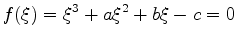 . . |
|
The factor of  can always be normalized to 1 since we can
divide through by the highest coefficient. Moreover, the absolute
term can always be made negative because, if it is originally
positive, we put
can always be normalized to 1 since we can
divide through by the highest coefficient. Moreover, the absolute
term can always be made negative because, if it is originally
positive, we put
 and operate with
  .
.
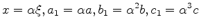
Now it is convenient to introduce a new scale factor which will
normalize the absolute term to  . We put
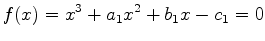
and write the new equation
If we choose
we obtain
Now, since  is negative and
 is positive, we know
that there must be at least one root between
is positive, we know
that there must be at least one root between  and
and  .
We put
.
We put  and evaluate
  . If
is positive, the root
must be between 0
and
. If
is positive, the root
must be between 0
and  ; if
is negative, the root must
be between
and
; if
is negative, the root must
be between
and  . Moreover, since
we know in advance that we cannot have three roots
between 0
and
, or
and
. Hence if  ,
we know that there must be one and only one real root
in the interval
,
we know that there must be one and only one real root
in the interval ![$ [ 0 , 1 ]$](img132.png) , while if
, while if  , we know
that there must be one and only one real root in the interval
, we know
that there must be one and only one real root in the interval
![$ [1 , \infty]$](img134.png) . The latter interval can be changed to the interval
. The latter interval can be changed to the interval
![$ [1,0]$](img135.png) by the transformation
by the transformation
which simply means that the coefficients of the equation change
their sequence:
Hence we have reduced our problem to the new problem:
find the real root of a cubic equation in the range
.
We solve this problem in good approximation by taking advantage of
the remarkable properties of the Chebyshev polynomials (cf. VII, 9)
which enable us to reduce a higher power to lower powers with
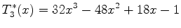
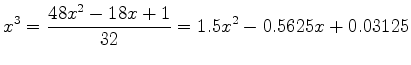
a small error. In particular, the third Chebyshev polynomial
normalized to the range
gives
with a maximum error of
 . The original cubic
is thus reducible to a quadratic with an error not exceeding
. The original cubic
is thus reducible to a quadratic with an error not exceeding
 .
.
We now solve this quadratic, retaining only the root between
0
and
.
11. Equations of fourth order.
Algebraic equations of fourth order with generally complex roots
occur frequently in the stability analysis of airplanes and in problems
involving servomechanisms.
The historical method of solving algebraic equations of fourth order
(also called biquadratic or quartic equations) involves the following
steps. By a transformation of the form
 the coefficient
of the cubic term is annihilated. Then an auxiliary cubic equation
is solved. The roots of the original equation are constructed with
the help of the three roots of the auxiliary cubic. Numerically
this method is lengthy and cumbersome. The following modification
of the traditional procedure yields the four roots of an arbitrary
quartic equation with real coefficients on the basis of a quick
and numerically convenient scheme.
the coefficient
of the cubic term is annihilated. Then an auxiliary cubic equation
is solved. The roots of the original equation are constructed with
the help of the three roots of the auxiliary cubic. Numerically
this method is lengthy and cumbersome. The following modification
of the traditional procedure yields the four roots of an arbitrary
quartic equation with real coefficients on the basis of a quick
and numerically convenient scheme.
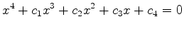
Every equation of the form
can be rewritten as follows:
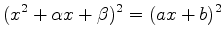 . . |
|
If the original  are real, the new coefficients are also real.
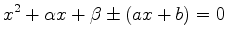
Hence the original equation becomes solvable in the form of the
quadratic equation
are real, the new coefficients are also real.
Hence the original equation becomes solvable in the form of the
quadratic equation
which has four (generally complex) roots, obtainable by the standard
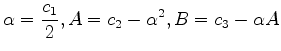
formula. The new coefficients can be determined as follows. We
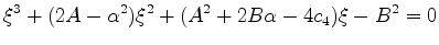
evaluate in succession the following numerical constants:
and form the cubic equation
Since the left side is negative at  , a positive real root
must exist. We determine this root according to the method of § 3.
In order to avoid later corrections, it is advisable to add at this point
Newton's correction (cf. § 5), obtaining
, a positive real root
must exist. We determine this root according to the method of § 3.
In order to avoid later corrections, it is advisable to add at this point
Newton's correction (cf. § 5), obtaining  with great accuracy.
The coefficients of the reduced equation are then determined as follows:
with great accuracy.
The coefficients of the reduced equation are then determined as follows:
|
|
|
|
| Two point raytracing for reflection off a 3D plane | |
|
Next: APPENDIX B
Up: APPENDIX A
Previous: APPENDIX A
2012-10-29


![$\displaystyle \vdots \makebox[0.9\textwidth][1pt]{\ } $](img142.png)