Decon in the log domain - practical considerations

Near offset

The dataset we used is a single 2D line from a marine streamer survey in the Gulf of Baja California (Lizzaralde et al., 2002). This line consists of 2298 shots. There were 480 receivers along the cable, and the group spacing was 12.5m. The nearest offset was 180m, and the farthest was 6180m.

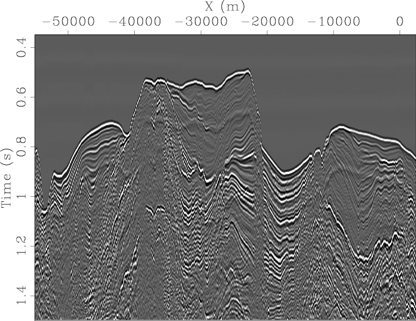
Figure 1 is the near-offset section of the data. A gain of $t^2$ has been applied. Note the Ricker-like appearance of the reflections. Note also the bubble visible 200ms below the sea-bottom reflection. Other weaker bubble reverberations are within the section. A weak direct arrival of one of the bubble reverberations appears faintly at 500ms.

We ran two types of inversions:

1. Gained input deconvolution: Inversion is applied to data which was gained by $t^2$ , and there is no gain applied to the residual $(g_t = t^0)$ .
2. Gained output deconvolution: Input data was not gained, but the residual was gained at each iteration of the inversion $(g_t = t^2)$ .

Additionally, for each gain type, we ran the inversion with and without regularizations, by setting the values of $\epsilon_1$ and $\epsilon_2$ in equations (2) and (3) accordingly.

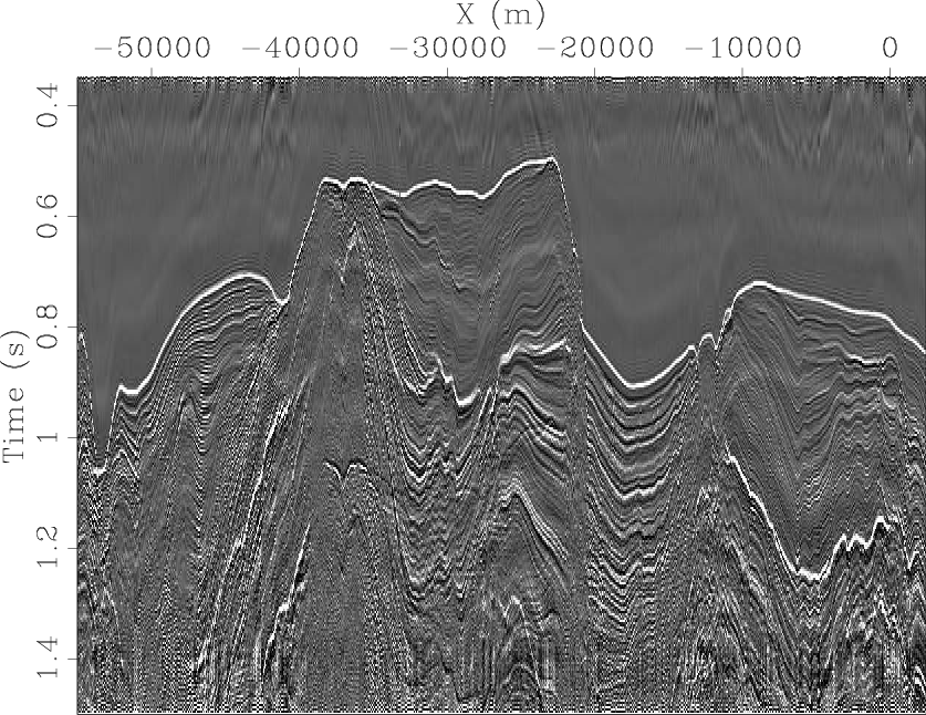
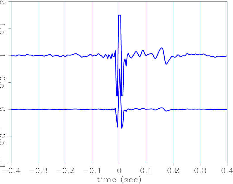
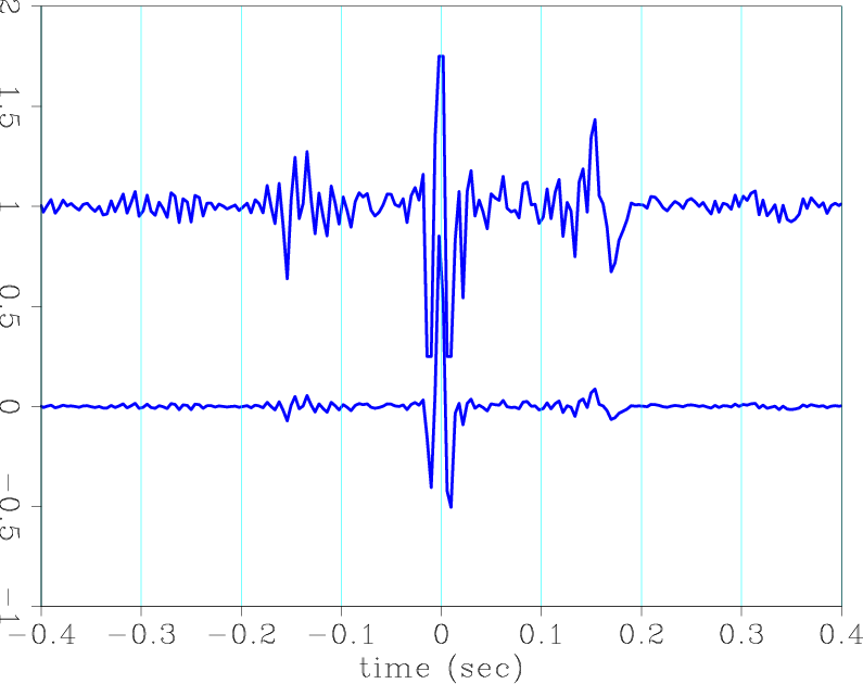
Figure 2(a) shows the gained input deconvolution run without regularizations. Note that while the deconvolution has indeed spiked the reflections on the central lobe of the Ricker wavelet, the bubble is still visible, and the precursors are strong. Figure 2(b) is the gained output deconvolution run without regularizations. While the bubble seems to have been dealt with better in this section, the precursors above the sea-bottom reflection are stronger, and the entire section appears noisier. Figure 4(a) shows the shot-waveform estimated by the gained input deconvolution, and 4(b) is the one estimated by the gained output deconvolution. In each plot, the upper trace is the same as the lower trace, except that it has been clipped in order to enhance the smaller coefficients in the display. The smaller coefficients are important, since deconvolution is a division operation. Note how much more energy is in the anti-causal part of the shot-waveform in Figure 4(b) as compared to Figure 4(a). Both of them however show the main shot-waveform as a Ricker centered at zero-lag, and a bubble with its associated reverberations. This means that the inversion has indeed arrived at what we assumed to be the correct objective: in order to sparsify the data, the Ricker wavelet and the bubble must be removed.

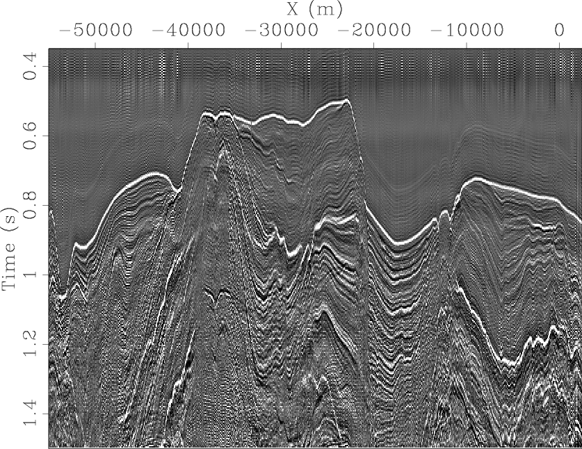
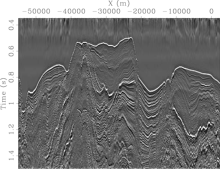
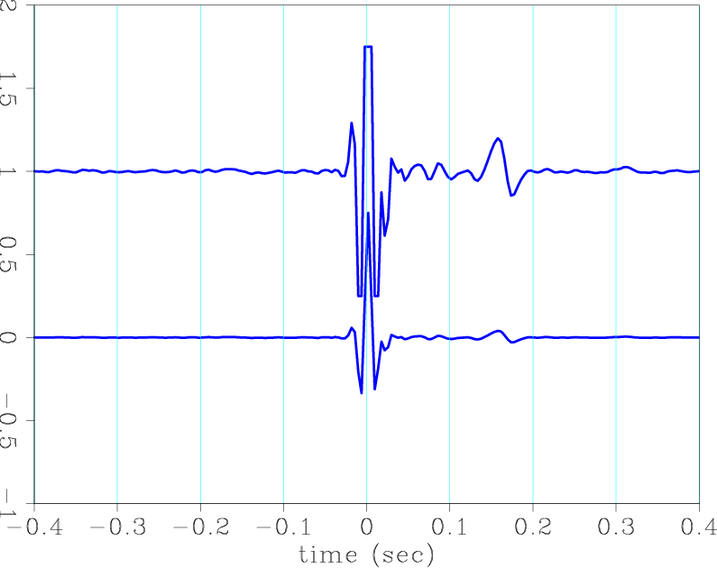
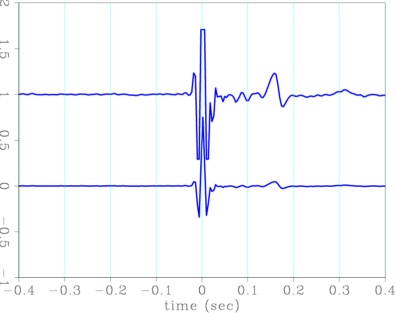
Figure 3(a) is the gained input deconvolution run with the symmetry and filter length regularizations. Compared to Figure 2(a), the bubble is weaker, and so are the precursors. This can be further validated by comparing the precursors of the shot waveform in Figure 4(a) vs. Figure 4(c). Figure 3(b) is the gained output deconvolution run with the regularizations. Compared to Figure 3(a), the bubble is better eliminated. There is a slight difference in the estimated bubble in the shot-waveforms of Figures 4(c) and 4(d), and this is enough to cause the difference in bubble elimination. The precursors for the gained output deconvolution with regularization are the weakest, which is a direct result of forcing the filter length to be short.

EW05s
Figure 1. Gained near-offset section of Baja data. Offset is 180m. Note the Ricker-like appearance of the reflections, and the bubble around 200ms below the sea-bottom reflection.

deconEW05s-t0-6,deconEW05s-t2-6
Figure 2. Deconvolution of the 180m offset only. (a) Gained input deconvolution without regularization. (b) Gained output deconvolution without regularization. Note how the Ricker wavelet has been spiked, and the strong precursors.

deconEW05s-t0-reg-6,deconEW05s-t2-reg-6
Figure 3. Deconvolution of the 180m offset only. (a) gained input deconvolution with regularization. (b) gained output deconvolution with regularization. Compared to Figures 2(a) and 2(b), the precursors are weaker and the bubble is better handled. In (b) there is less noise than in (a).

EW05s-t0-6,EW05s-t2-6,EW05s-t0-reg-6,EW05s-t2-reg-6
Figure 4. Estimated shot waveforms resulting from inversion using near offset data only. In each graph, the lower trace is unclipped, and the upper trace is clipped to enhance the small coefficients. (a) Gained input decon without regularization (link to figure 2). (b) Gained output decon without regularization. (a) and (b) are the shot waveforms, and their inverses are those that generated Figures 2(a) and 2(b) after deconvolution. Note how much more energy is in the anti-causal part of the shot waveform in (b) compared to (a). (c) Gained input decon with regularization. (d) Gained output decon with regularization. (c) and (d) are shot waveforms, the inverses of which generated Figures 3(a) and 3(b) after deconvolution.

Decon in the log domain - practical considerations