|
|
|
|
Efficient depth extrapolation of waves in elastic isotropic media |
The system of matrix equations 8 is solved only once for each triple of temporal frequency and elastic moduli values, and for each pair of horizontal wave numbers. In our prototype implementation of the one-way extrapolator we compute the matrices  at the beginning of the frequency loop and subsequently use the tabulated matrices in the depth extrapolation loop (inside the frequency loop). A more efficient approach can be employed in a production implementation of the extrapolation method: system 8 can be solved using Newton's method (see e.g. (Higham, 2008)) in a one-off computation for each set of the temporal frequency, elastic moduli and horizontal wave numbers and stored in a look-up table. The symmetry of the extrapolation operators 11, that appear to be multi-component counterparts of the acoustic phase-shift operator (see Claerbout (1985)), can be exploited to achieve a substantial reduction in the size of the precomputed operator tables. Figure 1 is the plot of the maximum of the imaginary parts of the three eigenvalues of operator
 , of equation 15, is the logarithm of the extrapolation operator 11, and the spectral plot of Figure 1 corresponds to the phase of the phase-shift extrapolator in the acoustic case (see (Biondi, 2005)). The crucial difference in the elastic multicomponent case is that the multicomponent ``phase-shift'' is defined by three such scalar phase-shift operators with phases
 , and a unitary operator
 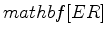 , determined by the eigenvector expansion of
as follows:
, determined by the eigenvector expansion of
as follows:
The pass bands of the three phase shift operators are, generally, different, but the real parts of the eigenvalues of 15 are non-positive across all three pass bands.
Figures 2,3,4,5 demonstrate the result of applying our method to extrapolating displacement waves from a concentrated impulse at the surface. Medium parameters used in this test were  m/s shear-wave velocity

and
 m/s pressure-wave velocity

The extrapolation grid was
 with a 5 m step, frequency range 2-12 Hz with 1 Hz step. The values of the elastic parameters used in this test are uncharacteristically low for seismic applications and were chosen solely for the purpose of fast small-scale simulation on a single-core PC using Matlab.
|
pressure
Figure 2. Pressure wave extrapolated from an impulse displacement, 2-12 Hz,
grid,  m step,
m/s shear-wave and
m/s pressure-wave velocity.
m step,
m/s shear-wave and
m/s pressure-wave velocity.
|
|
|---|---|
|
|
|
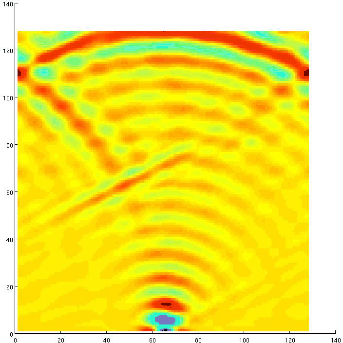
component3
Figure 3. Vertical component of a wave extrapolated from an impulse displacement, inline section, 2-12 Hz,  grid,
m step,
m/s shear-wave and
m/s pressure-wave velocity.
grid,
m step,
m/s shear-wave and
m/s pressure-wave velocity.
|
|
|---|---|
|
|
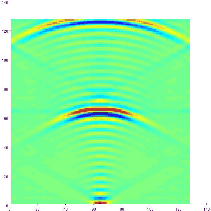
Since the impulse at the surface is an asymmetric horizontal displacement but can be assumed to be symmetric in the vertical direction, our waves are effectively a combination pressure and shear waves for the horizontal components, while the vertical displacement wave should kinematically match the pressure wave. And indeed, the pressure wave plot 2 and vertical displacement plot 3 exhibit excellent kinematic agreement.
|
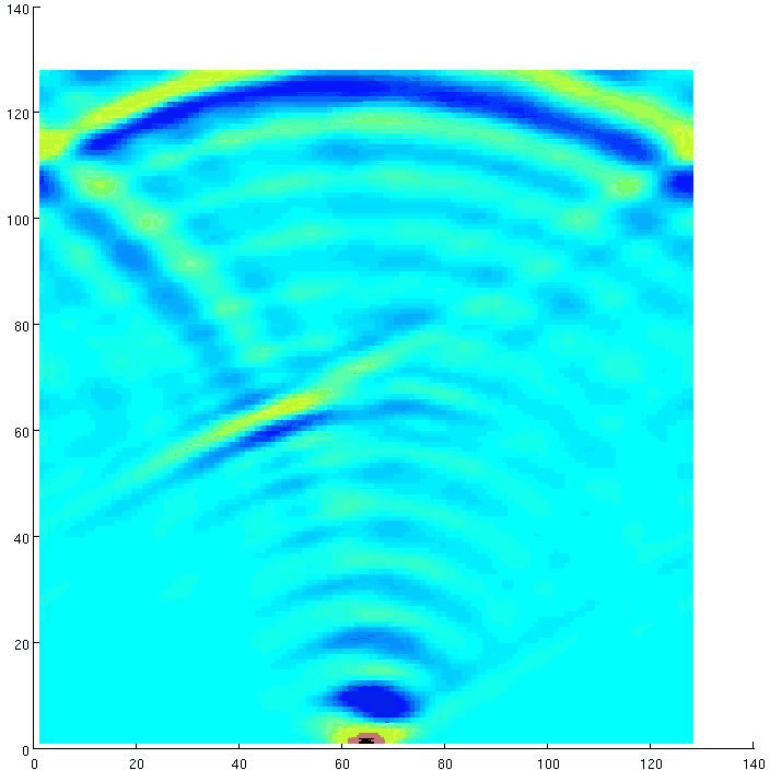
component1
Figure 4. Inline component of a wave extrapolated from an impulse displacement, inline section, 2-12 Hz,
grid,
m step,
m/s shear-wave and
m/s pressure-wave velocity. Note the slow shear wave.
|
|
|---|---|
|
|
|
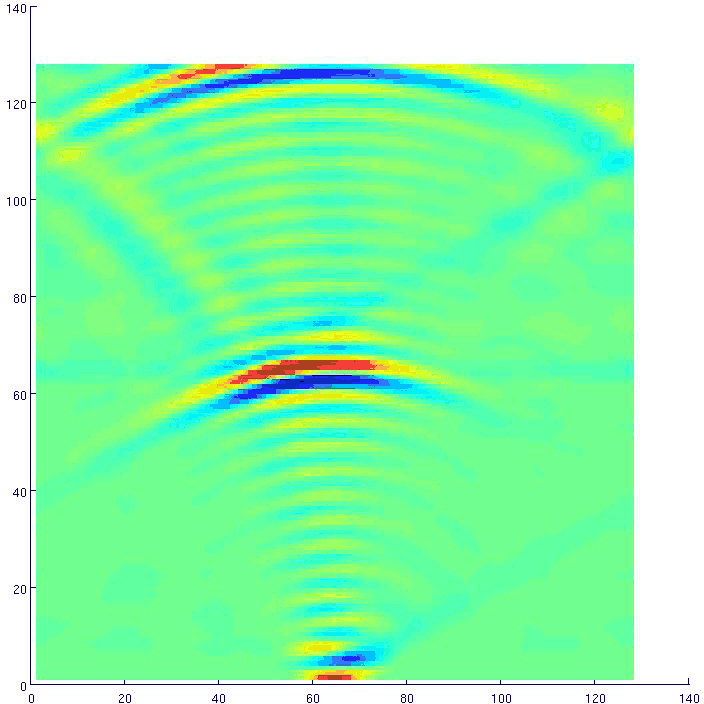
component2
Figure 5. Crossline component of a wave extrapolated from an impulse displacement, inline section, 2-12 Hz,
grid,
m step,
m/s shear-wave and
m/s pressure-wave velocity. Note the slow shear wave.
|
|
|---|---|
|
|
The horizontal wave-component plots 4 and 5, on the other hand, show pressure- and shear-wave images, both correctly positioned in agreement with the velocity values used in the simulation. Boundary reflections and low frequency content cause some imaging artifacts that are not related to the method.
|
|
|
|
Efficient depth extrapolation of waves in elastic isotropic media |
![$\displaystyle K=-\Delta z E^{-1}\left[A(-i\partial_x,-i \partial_y)+c_{\omega}I\right],$](img59.png)
![$\displaystyle K=Q\left[ \begin{array}{ccc} i\phi_1 & 0 & 0 \\ 0 & i\phi_2 & 0 \\ 0 & 0 & i\phi_3 \end{array} \right]Q^{\ast}.$](img62.png)