Tomographic full waveform inversion and linear modeling of multiple scattering

Problems with FWI

Unfortunately, high-order scattering must be taken into account to model accurately wavefield perturbations when the velocity perturbations have wide spatial extent and/or large amplitude. Such velocity perturbations cause significant (larger than one fourth of wave cycle) time shifts in the propagating wavefield. The linear operator ${\bf L}$ cannot model large time shifts because the source function on the right-hand side of equation 8 is triggered by the background wavefield reaching a velocity perturbation, and consequently it has the timing as the background wavefield. Furthermore, the perturbed wavefield is propagated with the background velocity ${\bf {v}_o}$ . In mathematical terms

$${\cal L}\left({\bf {v}_o}^2 + \delta{{\bf {v}}}^2\right) \neq {\c... ...t({\bf {v}_o}^2\right) + {\bf L}\left({\bf {v}_o}^2\right) \delta{{\bf {v}}}^2.$$ (9)

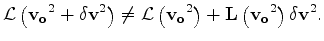
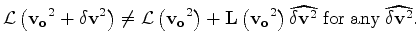
The problem is even deeper. When $\delta{{\bf {v}}}^2$ causes large time shifts by multiple scattering, there is no perturbation $\widehat{\delta{{\bf {v}}}^2}$ that can model those time shifts by single scattering; that is,

$${\cal L}\left({\bf {v}_o}^2 + \delta{{\bf {v}}}^2\right) \neq {\c... ...idehat{\delta{{\bf {v}}}^2} \;{\rm for\; any \;} \widehat{\delta{{\bf {v}}}^2}.$$ (10)

The non linearity of the modeling operator makes the objective function equation 2 to be non convex when the velocity perturbations are sufficiently large. Figure 1 shows an example of non-convexity of the objective function. The result correspond to several 1D transmission problems sharing the same starting velocity (1.2 km/s) and with different true velocities. For all these experiments the source-receiver offset is 4 km and the source function is a zero-phase wavelet bandlimited between 5 and 20 Hz. The FWI norm is plotted as a function of the true velocity. If the true velocity is lower than $\approx 1.18$ km/s or larger than $\approx 1.22$ km/s a gradient based method will not converge to the right solution, even in this simple and low-dimensionality example.

The challenges of solving the optimization problem in equation 1 by gradient based optimization can be alternatively represented by graphing, as a function of the initial velocity error, the search direction (opposite sign of the gradient direction) of the objective function with respect to velocity square. Figure 2 display this function computed by applying the adjoint of the linear operator ${\bf L}$ to the data residuals; that is

$$\nabla {J_{\rm FWI}}= {\bf L}' \left[ {\cal L}\left({\bf {v}_o}^2\right) - {\bf d} \right].$$ (11)

For a gradient based method to converge, the search direction should be always negative when the true velocity is lower than 1.2 km/s, and positive when the true velocity is higher.

Tomographic full waveform inversion and linear modeling of multiple scattering