|
|
|
|
Tomographic full waveform inversion and linear modeling of multiple scattering |
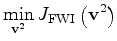
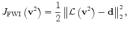
 is the velocity vector,
 is a wave-equation operator non linear with respect to velocity
perturbations and
the data vector
is a wave-equation operator non linear with respect to velocity
perturbations and
the data vector  is the pressure field
 measured at the surface.
The wave-equation operator is evaluated by recursively solving the following finite difference equation
 is a finite-difference representation of the second derivative in time,
 is a finite-difference representation of the Laplacian,
and
is a finite-difference representation of the Laplacian,
and  is the source function.
|
|
|
|
Tomographic full waveform inversion and linear modeling of multiple scattering |
![$\displaystyle \left[ {\bf D_2}- {\bf {v}}^2\nabla^2 \right] {\bf P} ={\bf f},$](img9.png)