|
 |
 |
 | Six tests of sparse log decon |  |
![[pdf]](icons/pdf.png) |
Next: Data plots
Up: Guitton and Claerbout: Sparse
Previous: INTRODUCTION
Because predictive decon fails on the Ricker wavelet,
Zhang and Claerbout (2010)
devised an extension to non-minimum phase wavelets.
Then Claerbout et al. (2011)
replaced the traditional unknown filter coefficients
by lag coefficients  in the log spectrum of the deconvolution filter.
Given data
in the log spectrum of the deconvolution filter.
Given data  , the deconvolved output is
![$\displaystyle r_t \ =\ {\rm FT}^{-1}\ \left[ D(\omega)\ \exp\left( \sum_t u_tZ^t \right) \right]$](img6.png) |
(1) |
where
 .
The log variables
transform the linear least squares (
.
The log variables
transform the linear least squares ( ) problem
to a non-linear one that requires iteration.
The gained residual
) problem
to a non-linear one that requires iteration.
The gained residual
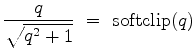
 is ``sparsified''
by minimizing
is ``sparsified''
by minimizing
 where
where
Traditional decon approaches are equivalent to choosing a white spectral output.
Here we opt for a sparse output.
Earlier frustrations led to various regularizations.
We minimize the following functional:
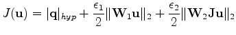 |
(5) |
where bold faces are for either vectors or matrices.
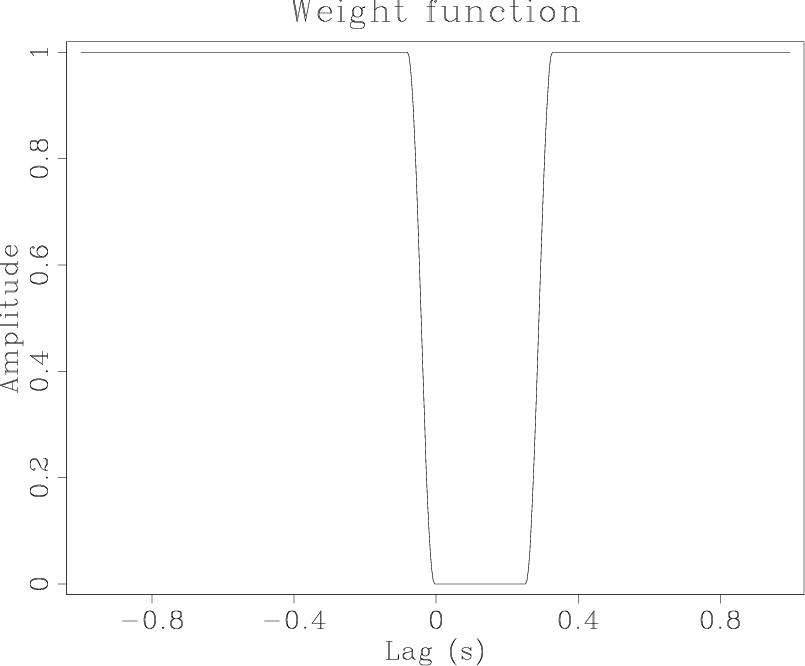
The first regularization term tends to limit the range
of filter lags (Figure 1).
The second term, introduced by Claerbout et al. (2012)
encourages symmetry
(
 ) around the central Ricker lobe.
It does this by a matrix
) around the central Ricker lobe.
It does this by a matrix  that senses asymmetry
 at small lags
  and suppressing it.
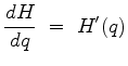
The gradient search direction becomes
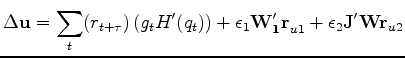 |
(6) |
It happened in all the examples in this paper
(except the one with a defective airgun array)
the
 ``Ricker regularization'' was not needed
because no polarity reversals or apparent time shifts were noted so
``Ricker regularization'' was not needed
because no polarity reversals or apparent time shifts were noted so
 in all cases.
The value of
in all cases.
The value of
 was selected by trial and error.
Weight
Figure 1.
Weighting function used in the regularization to force long lags
to be zero. The positive lags allow more non-zero coefficients
to include the bubble.
These limits apply in the lag-log space of  and so apply only approximately to the shot waveform and the decon filter.
|
|
![[png]](icons/viewmag.png)
|
|---|
Subsections
|
|
|
|
| Six tests of sparse log decon | |
|
Next: Data plots
Up: Guitton and Claerbout: Sparse
Previous: INTRODUCTION
2012-10-29