Fast log-decon with a quasi-Newton solver

A comparison on a field-data example

Figure 1 shows a near-offset section of a 2-D line from the Gulf of California used in Claerbout et al. (2012). The left side displays the input data and the right side the deconed data when the L-BFGS solver is used. I do not show the result of the steepest-descent because both methods estimate very similar wavelets, as shown in Figure 2. As expected, the reflectivity of the deconed data in Figure 1 is revealed quite well: the polarity of large reflectors is enhanced. Also, a non-minimum phase wavelet is obtained, regardless of the method (Figure 2).

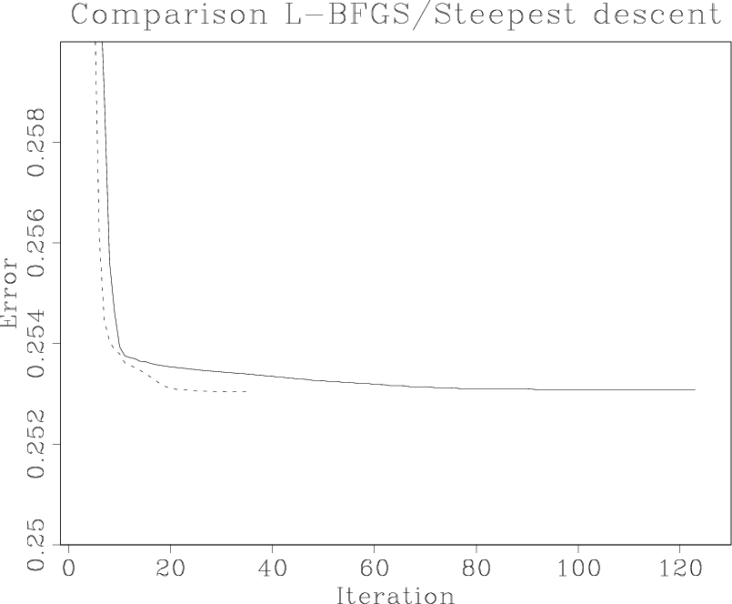
In terms of convergence speed, it takes 35 iterations and 1.7 seconds for the L-BFGS technique to reach a minimum, and 123 iterations and 24 seconds for the steepest-descent algorithm (Figure 3). Ignoring the time it takes to read and write data on disk, each iteration of the L-BFGS algorithm is about five times faster, with almost four times less iterations. Clearly, this difference is not solely due to the better convergence properties of the quasi-Newton algorithm over the steepest-descent method. As mentioned before, different line-search strategies and stopping criteria matter as well.

Comp-cabo
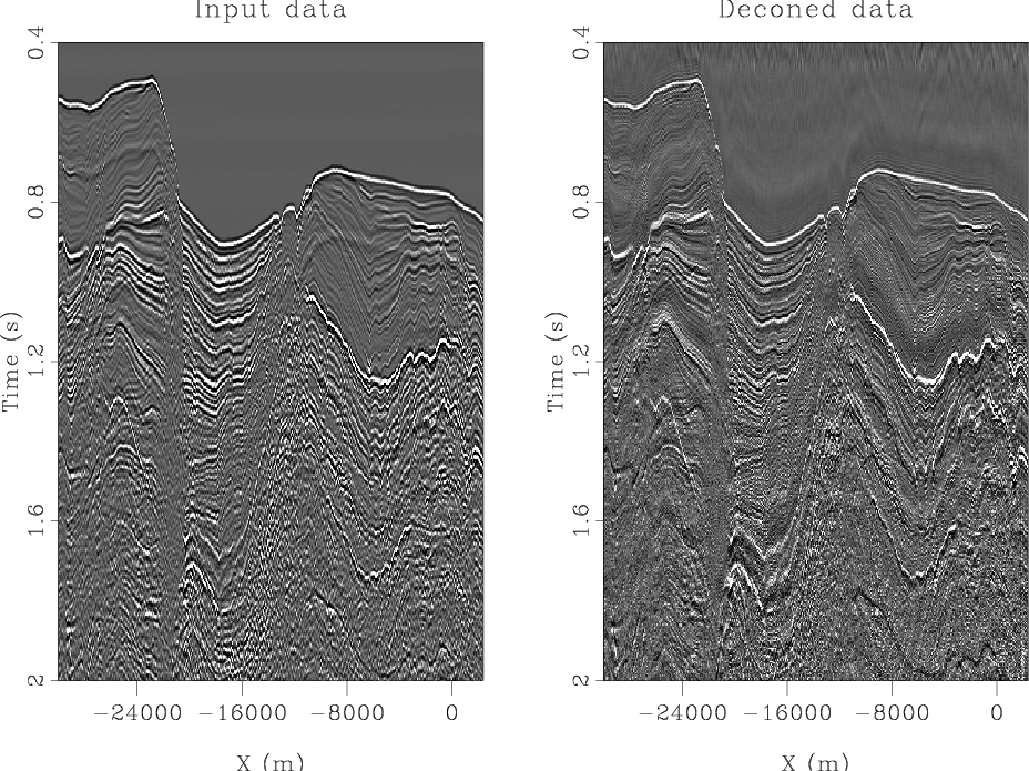
Figure 1. Left: input data. Right: deconed data with the L-BFGS solver

Comp-wvlt
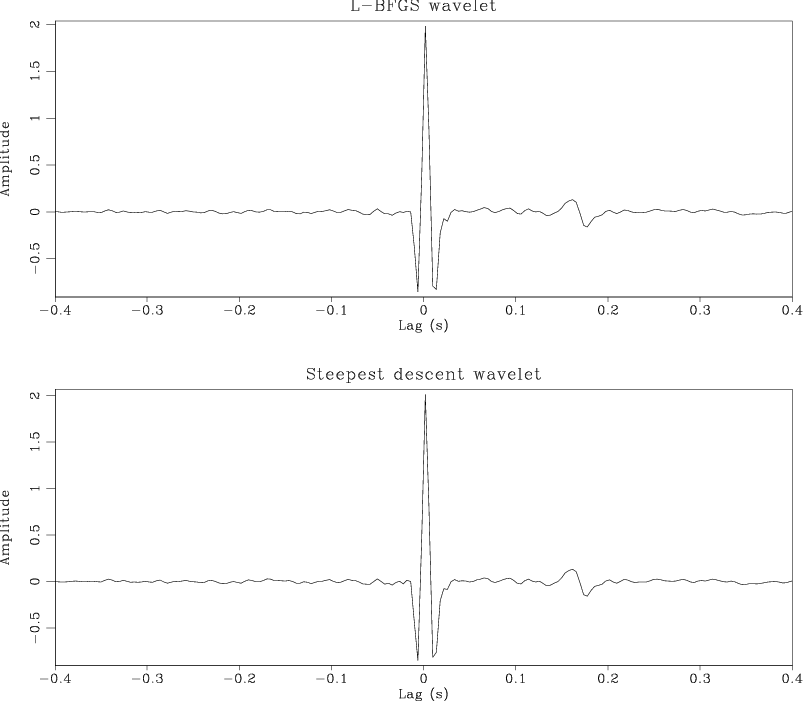
Figure 2. Top: wavelet estimated with the L-BFGS method. Bottom: wavelet estimated with the steepest-descent method.

Comp-fct Figure 3. Convergence comparison between the steepest descent (solid) and L-BFGS (dash) methods. Note the narrow horizontal scale to highlight small differences close to the convergence point.

Fast log-decon with a quasi-Newton solver