Computational analysis of extended full waveform inversion

Synthetic Examples

A modified Marmousi model is used for the synthetic example where a 500m water layer is added to the top. Figure 4 shows the true velocity model. A Ricker wavelet with a fundamental frequency of 15 Hz and temporal sampling of 1.5 ms is used as a source function to model the data. 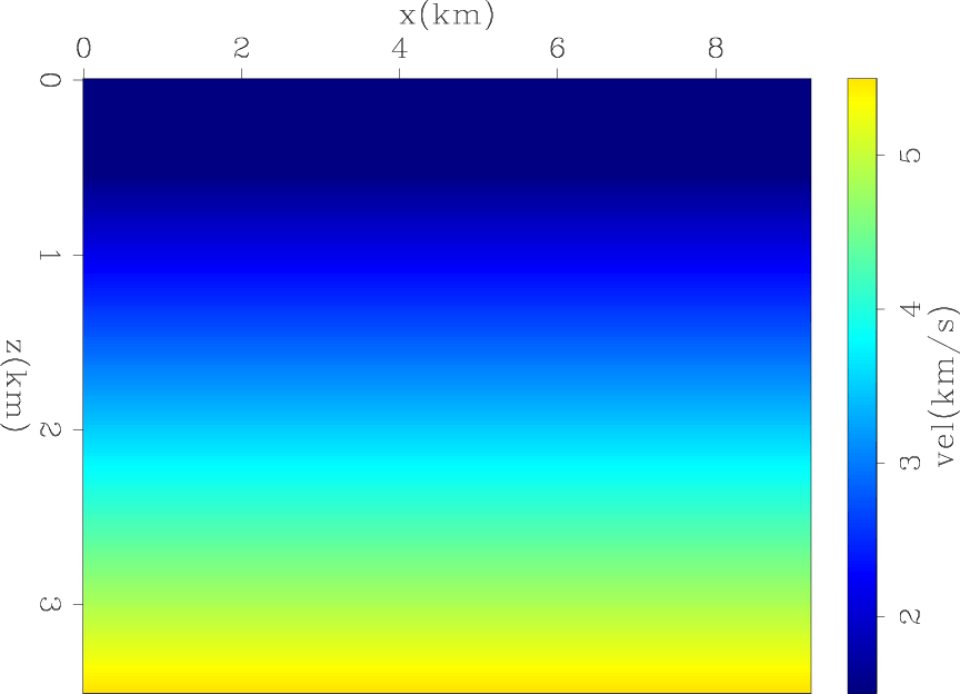There are 461 fixed receivers with a spacing of 20 m and 21 plane sources with ray parameter ranging from $-1$ s/km to $1$ s/km. The initial model shown in Figure 5 is obtained by strongly smoothing the true model.

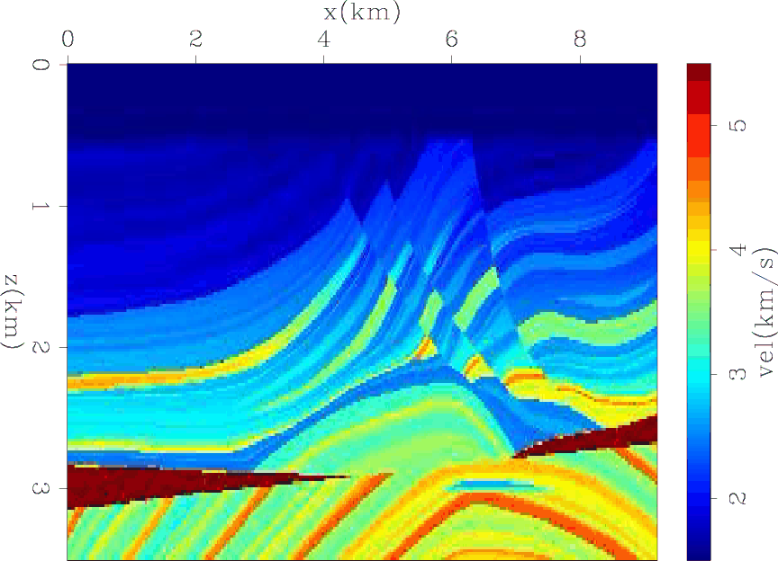
vtrue Figure 4. The true velocity of Marmousi model.

init Figure 5. The initial velocity of Marmousi model.

I modeled the observed data with the conventional acoustic wave-equation nonlinear modeling operator. Then, I ran inversion without any tomographic regularization term. This inversion verified the first extension condition, that the modeled data can be explained using the initial model.

res2 Figure 6. The data residual norm as a function of iterations of Marmousi model unregularized inversion.

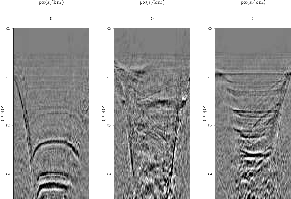
inv2dv Figure 7. Three ray parameter gathers showing the difference between the initial model and the unregularized inverted model at x=2.5, 5, 7.5 km of Marmousi model.

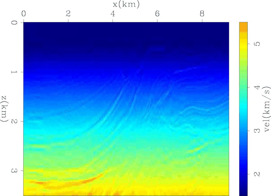
inv2 Figure 8. The unregularized inversion results of Marmousi model.

I show the results of running 1000 iterations of the unregularized inversion. Figure 6 shows the residual of the data fitting as a function of iterations. The residual decreases monotonically without getting stuck in a local minima and is approaching zero. This means that the first condition is fairly satisfied for this example. Figure 7 shows the difference between the initial and final model at three locations as a function of depth and ray parameter. The three gathers show varying degrees of difference across the ray parameter axis, which indicates the inconsistency between these data components given the initial velocity model. Figure 8 shows the average of the final model across the ray parameter axis. Although the final model matches most of the observed data, no low wavenumber components are correctly estimated in this unregularized inversion since the kinematic errors are compensated for by the difference between ray parameter models.

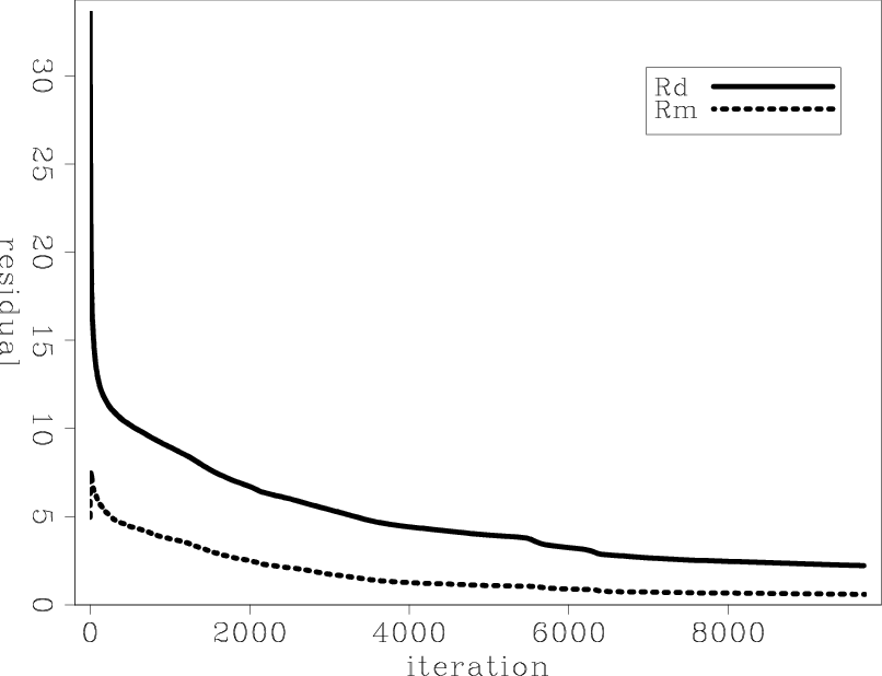
res Figure 9. The data residual norm (solid line) and the model residual norm (dashed line) as a function of iterations of Marmousi model regularized inversion.

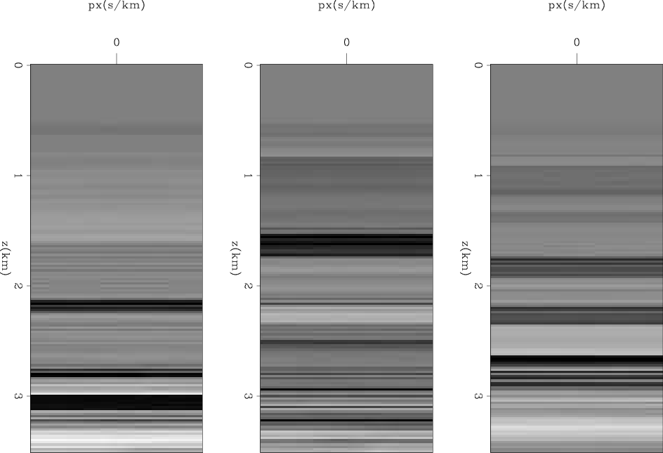
invdv Figure 10. Three ray parameter gathers showing the difference between the initial model and the regularized inverted model at x=2.5, 5, 7.5 km of Marmousi model.

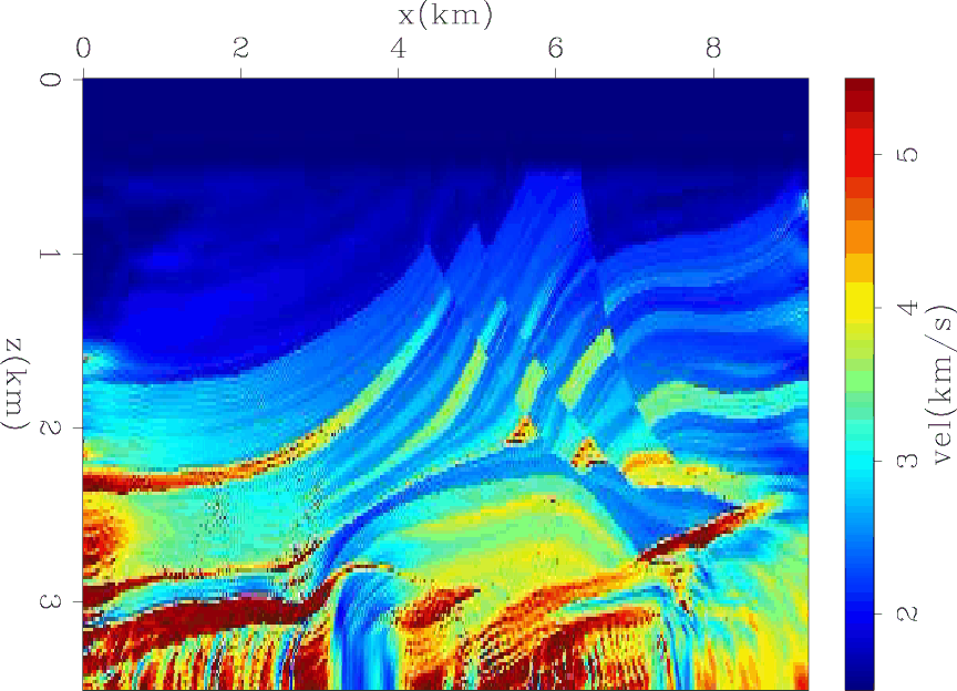
inv Figure 11. The regularized inversion results of Marmousi model.

Next, I show the results of running 10000 iterations of the inversion regularized by a derivative across the ray parameter axis. Figure 9 shows the residual of the data fitting and model regularization as a function of iterations. The data fitting residuals decrease slower than the data residuals in the unregularized inversion since two objective functions are competing to be minimized. Nonetheless, it is not getting stuck in a local minima and is approaching zero. Figure 10 shows the difference between the initial and final model at three locations as a function of depth and ray parameter. The three images show no variations across the ray parameter axis, which indicates that the inversion successfully converged the extended model to a physical model. Figure 11 shows the average of the final model across the ray parameter axis. Both low and high wavenumber components are correctly estimated and the inversion converged towards the true answer.

Computational analysis of extended full waveform inversion