next up previous [pdf]

Next: Data-Space Extensions Up: Computational Cost Previous: Model-Space Extensions

Linearized Model-Space Extensions

Any of the previously mentioned inversions can be linearized by scale separation as shown in Almomin and Biondi (2012). To linearize the conventional FWI, the velocity model is separated as:

$\displaystyle s^{2}(\mathbf x) = b(\mathbf x) + r(\mathbf x),$ (14)

where $ b(\mathbf x)$ 
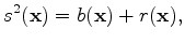
is the background component and $ r(\mathbf x)$ 
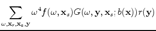
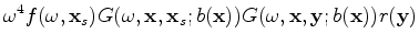
is the perturbation component. The linearized FWI forward operator can be written as follows:

$\displaystyle d(\omega, \mathbf x_r, \mathbf x_s; b(\mathbf x), r(\mathbf x)) =...
..._r; b(\mathbf x)) r(\mathbf x) G(\omega, \mathbf x, \mathbf x_s; b(\mathbf x)).$ (15)

As shown in equation 15, the cost of the linearized forward operator is equal to the adjoint cost of conventional FWI. Also, the adjoint of the linearized operator with respect to the perturbation is the same as the conventional FWI adjoint and has the same cost as well. The adjoint with respect to the background is:

$\displaystyle \Delta b(\mathbf x) =$ $\displaystyle \sum_{\omega, \mathbf x_r, \mathbf x_s, \mathbf y} \omega^4 f(\omega, \mathbf x_s) G(\omega, \mathbf y, \mathbf x_s; b(\mathbf x)) r(\mathbf y)$    
  $\displaystyle G(\omega, \mathbf x, \mathbf y; b(\mathbf x)) G(\omega, \mathbf x...
... x)) \Delta d^*(\omega, \mathbf x_r, \mathbf x_s; b(\mathbf x), r(\mathbf x)) +$    
  $\displaystyle \omega^4 f(\omega, \mathbf x_s) G(\omega, \mathbf x, \mathbf x_s; b(\mathbf x)) G(\omega, \mathbf x, \mathbf y; b(\mathbf x)) r(\mathbf y)$    
  $\displaystyle G(\omega, \mathbf y, \mathbf x_r; b(\mathbf x)) \Delta d^*(\omega, \mathbf x_r, \mathbf x_s; b(\mathbf x), r(\mathbf x)).$ (16)

Although equation 16 has six Green's functions, only four propagations are required since each background wavefield is the same for two Green's functions. In addition, these background wavefields are the same for the adjoint of perturbation. Hence, the total cost of the linearized FWI per iteration, assuming complete reuse of background wavefields, is

$\displaystyle C_{\rm LFWI} = N_x N_y N_z N_{\rm source} (12 \times N_{tp} C_{\rm FDTD} + 12 \times N_{tp} + 9 \times N_{ti}).$ (17)

This shows that scale separation by itself increases the cost of the original nonlinear operator since it adds several propagations, imaging and scattering steps. However, a significant cost cutting for extended inversions is possible by extending only the perturbation component without extending background component. By following the same derivation for linearized FWI, I find the cost of linearized extended FWI in subsurface offset when I extend perturbation only to be

$\displaystyle C_{\rm LEFWI} = N_x N_y N_z N_{\rm source} (12 \times N_{tp} C_{\rm FDTD} + 12 \times N_{tp} + 2 \times N_{ti} + 7 \times N_{ti} N_{hx} N_{hy}).$ (18)

By extending only the perturbation, we remove the subsurface offset multiplication factor $ N_{tp}$ . This results in a large reduction in cost because the number of propagation time steps $ N_{tp}$ 
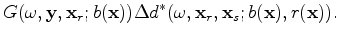
is much larger than the number of imaging time steps $ N_{ti}$ . Similarly, the cost of linearized extended FWI in time can be written as

$\displaystyle C_{\rm TimeLEFWI} = N_x N_y N_z N_{\rm source} (12 \times N_{tp} C_{\rm FDTD} + 12 \times N_{tp} + 2 \times N_{ti} + 7 \times N_{ti} N_{\tau}).$ (19)

For the extended FWI in time, the cost reduction by linearization is less dramatic than the extended FWI in subsurface offset since there is only one additional convolution axis.


next up previous [pdf]

Next: Data-Space Extensions Up: Computational Cost Previous: Model-Space Extensions

2012-10-29