|
|
|
|
Computational analysis of extended full waveform inversion |
 is subsurface offset and
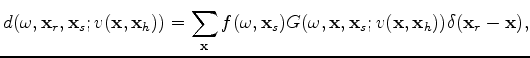
  denotes a deconvolution operator over subsurface offset. This extended wave equation convolves each time slice by all subsurface offsets of velocity. The cost of extended forward modeling becomes:
 and
and  are number of subsurface offsets along the
  and
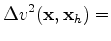
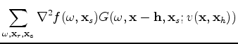
and  axes, respectively. By linearizing equation 7 over the velocity squared, we can compute the adjoint as:
 is the number of time lags. The computational disadvantage is that several time slices need to be held in memory for each time instead of the conventional two slices.
|
|
|
|
Computational analysis of extended full waveform inversion |