|
|
|
|
Estimation of Q from surface-seismic reflection data in data space and image space |
 is offset,
  is depth,
 , and
, and
 , which is a constant if I assume the velocity and the variance of the source are known.

|
|---|
|
trec50,trec99999,fpeak50,fpeak99999
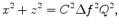
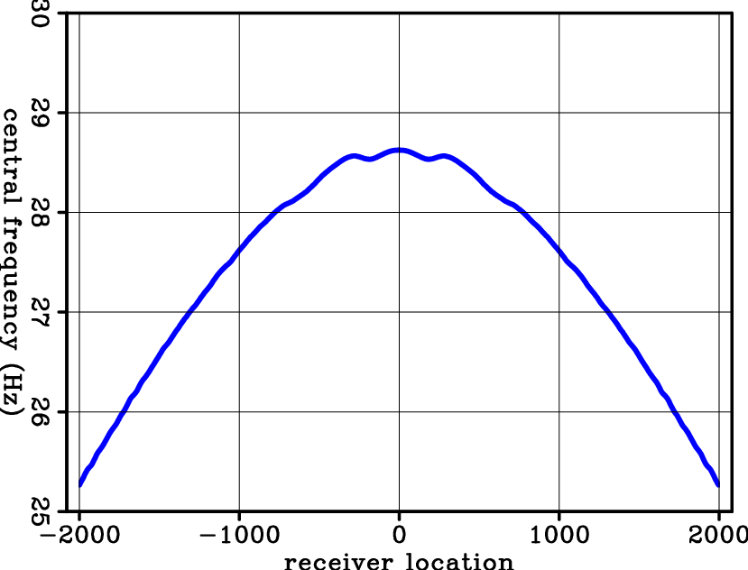
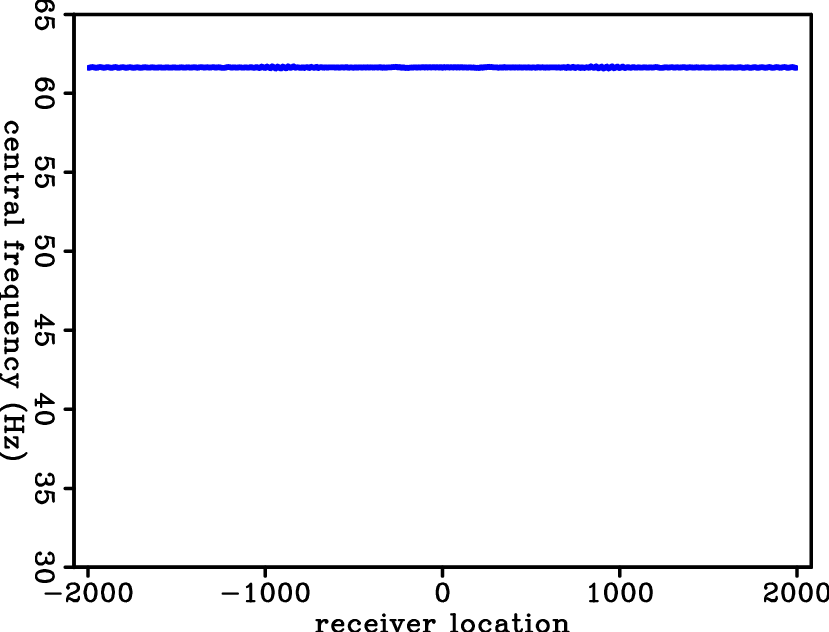
Figure 1. Given the 2D synthetic example, (a) modeled data with attenuation (Q=50); (b) modeled data without attenuation (Q=99999); (c) central frequency with attenuation; (d) central frequency without attenuation. |
|
|
Equation 10 relates four variables: two coordinates of the data space
 and two of the model space
  . An impulse in model space corresponds to a hyperbola in data space. In the opposite case, an impulse at a point in data space corresponds to another hyperbola in the model space. If I sum along the trajectories in the data space, energy will be concentrated in the model space to indicate the Q value. In this paper, I define the model space as the Q-spectra and the procedure described above as the Q-scan. Least-squares inversion can also be used here to yield a better result.
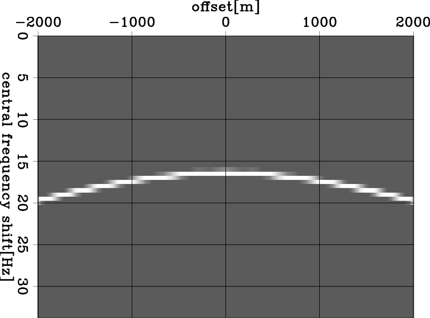
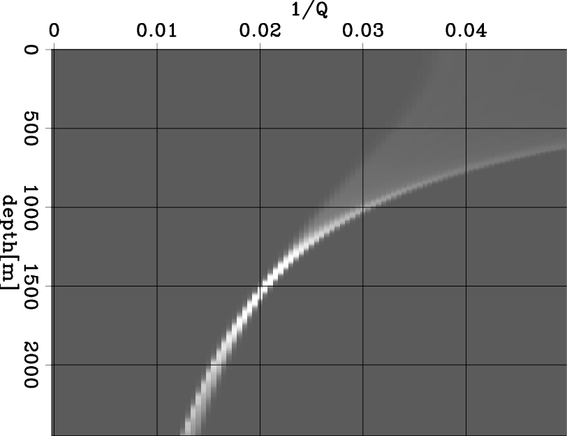
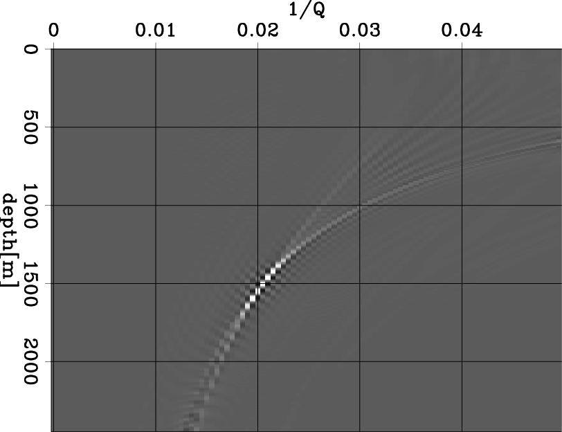
Figure 2(a) shows the central-frequency shift of the modeled data in Figure 1(a). After scanning, I compute the Q-spectra in Figure 2(b). This result shows concentrated energy around the expected point (1500 m, 0.02), which indicates that the RMS Q is 50 above 1500 m depth. Figure 2(c) shows least-squares inversion after 50 iterations. The energy is more focused on the expected point and shows much higher resolution. Therefore, I conclude that computing the Q-spectra can be used in estimating the RMS Q for a model with simple structure.
|
|---|
|
df,Qscanadj,Qscaninv
Figure 2. Figure 2(a) shows the central-frequency shift of the modeled data in Figure 1(a). The Q-spectra is computed in Figure 2(b). This result shows concentrated energy around the expected point (1500 m, 0.02), which indicates that the RMS Q is 50 above 1500 m depth. Figure 2(c) shows least-squares inversion after 50 iterations. The energy is more focused on the expected point and shows much higher resolution. |
|
|
In reality, however, this data-domain method can be inaccurate when lateral velocity variations and dipping structures exist. Therefore, image-domain methods is needed to more accurately estimate Q.
|
|
|
|
Estimation of Q from surface-seismic reflection data in data space and image space |