|
|
|
|
Early-arrival waveform inversion: Application to cross-well field data |
|
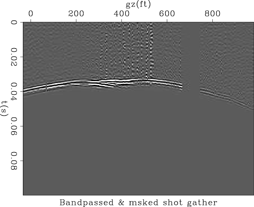
shotlpmsk
Figure 2. Same shot gather after bandpass and applying data mask. Data mask only keeps direct arrival for inversion purposes. |
|
|---|---|
|
|
Next we need to determine the proper source wavelet for forward modeling during inversion. Direct arrivals at the receiver side acurately represent what the source wavelet looks like. However, we are using two-dimensional modeling, whereas the field data source is a three-dimensional point source. We apply a phase shift to the direct arrival to correct for that. To improve the signal-to-noise ratio of the source wavelet, direct arrivals are first aligned by using picked first-break traveltime, then stacked to form the reference source wavelet. In this way, each shot has its own source wavelet. The original source and receiver coordinate has a  -ft interval increment. However, since our modeling grid has a
  -ft interval in both the
  and
and  directions, the source and receiver coordinates are rounded to a
-ft grid by nearest-neighbor criteria.
directions, the source and receiver coordinates are rounded to a
-ft grid by nearest-neighbor criteria.
The next element for waveform inversion is the starting model, which we obtain by using ray-based traveltime tomography. The tomography adopts the L2-regularized least-square approach to minimize the difference between observed and calculated traveltimes. We use the finite-difference Eikonal solver to compute the traveltime and then we back-project the raypaths from a receiver to the source (Zelt and Barton, 1998). We solve the objective equation by a Gauss-Newton strategy; for details see (Zhu and Harris, 2011). The observed data are the picked first break times from the full data set. The 2D inverse domain size is  by
by  cells, with a total number of 27,398 unknowns. The initial model for traveltime tomography has a constant velocity which is the average velocity value obtained from velocity logs. We ran ten iterations, stopping when the traveltime residuals were no longer significantly decreased. The final root-mean-square (RMS) residuals were reduced to 7.6e-3 ms from the initial value of 1.9 ms. Figure 3 shows the traveltime tomography result.
|
|---|
|
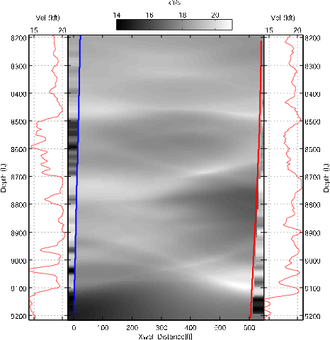
initmod
Figure 3. Starting model from traveltime tomography. Left line is receiver well. Right line is source well. Outside wells are well-log velocity values. |
|
|
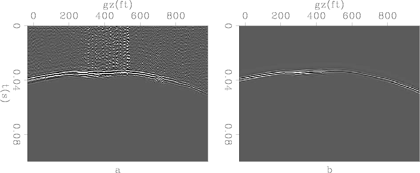
Comparison of data modeled from initial velocity and input data is shown in Figure 4. The finite difference modeling verified that the initial model predicts the data kinematics quite well in general. Only when traveltime is not continuous does the initial model have trouble producing a good match. Since the initial traveltime tomography result already matches picked first-break traveltime quite well, so the waveform inversion result mainly adds details to the traveltime tomography result.
|
|---|
|
initdatacomp
Figure 4. Same shot gather as before, comparsion of input first arrival and data modeled from the tomography result. The two are already very similar in terms of kinematics. a): Input first arrival; b): first arrival modeled from the tomography result. |
|
|
|
|
|
|
Early-arrival waveform inversion: Application to cross-well field data |