|
|
|
|
Early-arrival waveform inversion for near-surface velocity and anisotropic parameters: inversion of synthetic data |
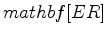 are laterally invariant, and value increases with depth (Figure 1 left column). Model perturbation consists of two symmetrical Gaussian anomalies in velocity, and one Gaussian anomaly in
(Figure 1 right column). The
anomaly is co-located with the left velocity anomaly. The true model consists of the background model plus the model perturbation. The starting model is the background model. Recorded early-arrival data using this model consists mostly of diving waves, and the model perturbation causes non-trivial traveltime perturbation in those waves, which is the major information used for updating the starting model.
are laterally invariant, and value increases with depth (Figure 1 left column). Model perturbation consists of two symmetrical Gaussian anomalies in velocity, and one Gaussian anomaly in
(Figure 1 right column). The
anomaly is co-located with the left velocity anomaly. The true model consists of the background model plus the model perturbation. The starting model is the background model. Recorded early-arrival data using this model consists mostly of diving waves, and the model perturbation causes non-trivial traveltime perturbation in those waves, which is the major information used for updating the starting model.
|
|---|
|
truemodsimpbw
Figure 1. Background model and model perturbation. a): background velocity model; b): velocity model pertubation; c): background
model; d):
model pertubation.
|
|
|
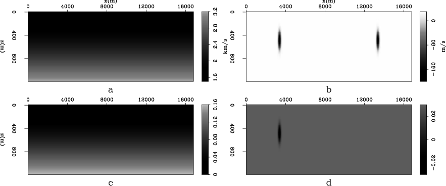
This is an ideal example to illustrate the ambiguity between velocity and
. I use the conventional L2 full waveform inversion (FWI) objective function (Tarantola, 1984), and vary the strength of the left velocity anomaly and the left
anomaly, while setting the strength of the right velocity anomaly to zero. A total of 64 shots with  -m spacing are modeled using the background model, with
  Hz peak source frequency. Since the radius of all anomalies is
  m, at a given source frequency, anomalies of this size mostly affect data traveltime rather than acting as a defractor. The traveltime differences are the major contributor to the objective function value. With receivers everywhere on the surface, the objective function value is shown in Figure 2 as a function of the two anomaly strength percentages. The valley in the center of the figure clearly indicates the ambiguity between velocity and anisotropy. If ambiguity exists even with such complete surface geometry, we can expect significant ambiguity in realistic acquisition scenarios. In such cases, proper model styling is needed in addition to data fitting.
|
|---|
|
fvalbw
Figure 2. Normalized objective function value as a function of percentage changes in the left vertical velocity anomaly and
anomaly strength. The vertical axis indicates the percent change in the vertical velocity anomaly. The horizontal axis indicates the percent change in the
anomaly.
|
|
|
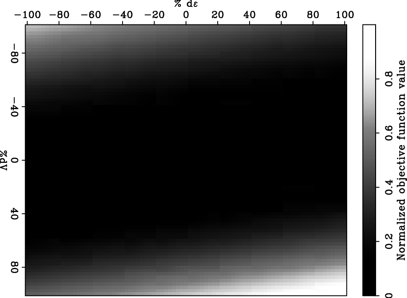
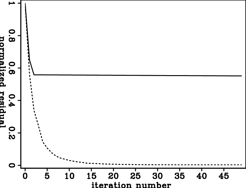
Inversion results using velocity parametrization are shown in the left column of Figure 3. Inversion results using logarithmic slowness parametrization are shown in the right column of Figure 3. Results from using logarithmic slowness parametrization are significantly better in terms of data misfit (Figure 4). However, even with very small data misfit, inversion results are still quite different from the true model. Such results also suggest the existence of ambiguity between vertical velocity and
in this simple example.
|
|---|
|
invdmodsimpbw
Figure 3. Inverted model perturbation. a): expressed in vertical velocity using velocity parametrization; b): expressed in vertical velocity using logarithmic slowness parametrization; c): expressed in
using velocity parametrization; d): expressed in
using logarithmic slowness parametrization.
|
|
|
|
|---|
|
resdsimpbw
Figure 4. Data residual as a function of iteration number during inversion using different inversion model parametrization. Continuous: velocity parametrization; dashed: logarithmic slowness parametrization. |
|
|
|
|
|
|
Early-arrival waveform inversion for near-surface velocity and anisotropic parameters: inversion of synthetic data |