Integral operator quality from low order interpolation or Sometimes nearest neighbor beats linear interpolation

Introduction

Many geophysical imaging and analysis tools involve summation over various trajectories within their input data. It is rare indeed that such summations do not involve intermediate interpolation among adjacent or nearby samples. Such interpolations are generally imperfect and so can degrade the final result--a subject of interest to me for some time (Levin, 1994). In a recent broad brush presentation of Kirchhoff time migration to an introductory C++ class at Stanford, I presented the slide:

and asserted

``Normally, an interpolator is selected based on its guaranteed-to-be-no-worse-than fidelity. However in the present case the distribution of many thousands or even millions of fractions of a sample to interpolate is uniform and so I focused in on the average rather than the worst case. From this perspective, looking at the amplitude behavior halfway between the 3rd and 4th curves plotted in the slide, the quite inexpensive linear interpolation does a good enough job in retaining fidelity. A similar plot of phase accuracy yields the same conclusion.''

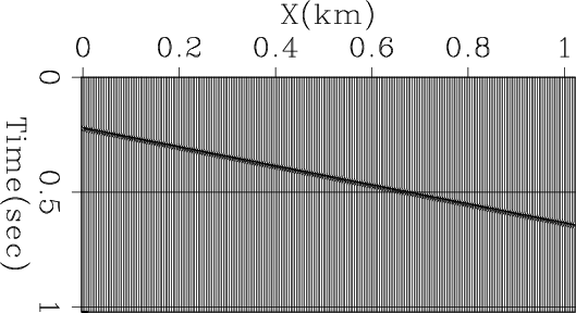
To understand this concept, let us take the very simple case of a single function replicated with linear delay and sampled with unit spacing as illustrated in Figure 1. Applying linear moveout and stacking would ideally reproduce that function. In order to apply the linear moveout we need to interpolate. Let us first consider what happens if we use simple nearest neighbor interpolation.

simpledip Figure 1. Simple dipping synthetic section.

We generally abhor nearest neighbor interpolation because it (a) is a discontinuous function of position and (b) can yield interpolated values that don't even have the correct sign. When stacking is included, though, to a good approximation we may assume the interpolation points are randomly distributed between samples following a uniform distribution. This means that the output values on our stack at are approximately

$$\int_{x_0-1/2}^{x_0+1/2} f(x) dx$$

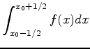which is convolutional filtering of $f(x)$ by a boxcar having Fourier transform

$$F(\omega) = (\omega / 2 )$$ (1)

Figure 2 illustrates the filter and its spectrum. Note that within the Nyquist limits $-\pi$ to $\pi$ , the spectrum (1) is positive, indeed greater than or equal to $2 / \pi$ . Therefore we can compensate for the nonflat spectrum by simple zero-phase spectral rebalancing after the stack, avoiding the expense of costly high quality sinc-like convolutions before stack.

nnint
Figure 2. Nearest neighbor boxcar filter (left) and its spectrum (right). Figure from Fomel (2000).

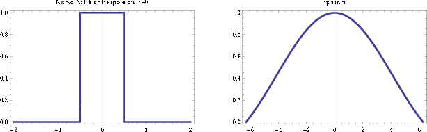
Seeing that nearest neighbor interpolation works unexpectedly well, let us turn our attention to linear interpolation. Following the same line of reasoning leads to a triangular convolution illustrated in Figure 3 which is a convolution of the nearest neighbor boxcar with itself and hence a spectrum that is the square of (1). This linear interpolation result is poorer than nearest neighbor, requiring more post-stack spectral compensation and concomitant noise magnification at higher frequencies!

linint
Figure 3. Nearest neighbor boxcar filter (left) and its spectrum (right). Figure from Fomel (2000).

Integral operator quality from low order interpolation or Sometimes nearest neighbor beats linear interpolation