P/S separation of OBS data by inversion in a homogeneous medium

Inverting for the virtual source model

The inversion is done by least-square fitting of modeled geophone data to the recorded geophone data. The model is a virtual-source array, injected into some locations in a homogeneous medium. There should be some distance between these virtual-sources' locations and the receiver line where the displacement fields will be recorded. This distance is necessary for the recreated wavefield to form.

It is not possible to recreate the entire original wavefield that was recorded by the geophones without accurate knowledge of the acquisition geometry and the medium parameters. However, given a particular acquisition geometry, and some reasonable medium parameters, it is possible to recreate the original wavefield in the vicinity of the geophones. This wavefield will form as a result of the injection of the virtual sources, and will become more similar to the originally recorded wavefield at the receiver locations as it propagates toward them.

The inversion starts from a zero-value initial model of displacement sources $\mathbf m^0 = \mathbf 0$ . This initial model is injected as a displacement force function, at locations $\mathbf x$ in the medium. The energy is propagated with the forward elastic operator, and recorded at locations $\mathbf y$ in the medium (the receiver locations):

$$\mathbf d = \mathbf {Fm^0}.$$ (18)

The residual that must be minimized is the difference between the calculated data $d$ , and the observed data $d_{\text{obs}}$ . The objective function is:

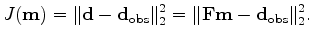$$J (\mathbf m) = \lVert \mathbf d - \mathbf d_{\text {obs}} \rVert^2_2 = \lVert \mathbf F \mathbf m - \mathbf d_{\text {obs}} \rVert^2_2.$$ (19)

The model gradient is:

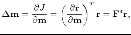$$\mathbf {\Delta m} = \frac{\partial J}{\partial \mathbf m} = \lef... ...ial \mathbf r}{\partial \mathbf m} \right)^T \mathbf r = \mathbf F^* \mathbf r,$$ (20)

where $\mathbf F^*$ is the adjoint elastic propagation operator. The data gradient is the forward operator applied to the model gradient:

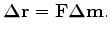$$\mathbf {\Delta r} = \mathbf F \mathbf {\Delta m}.$$ (21)

The model gradient and the data residual are updated using an itterative minimization scheme (Claerbout and Fomel, 2011).

The end result of the inversion is the model $\mathbf m$ which, when injected at locations $\mathbf x$ in a homogeneous medium with the parameters used in the inversion, will generate recorded data at locations $\mathbf y$ that are equal to the observed data. Even if the medium parameters that were used to generate the wavefield were not a good approximation to the true parameters, this difference will be minor with regard to the wavefield at a close proximity to the receivers. Therefore, if the data residual is zero, we can assume that the wavefield near the receivers has likewise been reliably recreated.

The displacement field values are calculated for all time steps by running the forward propagation operator using the final virtual-source model as an input:

$$F \begin{bmatrix}- \frac{1}{\rho} m_x \\ - \frac{1}{\rho} m_z \end{bmatrix} = \begin{bmatrix}u_x \\ u_z \end{bmatrix}.$$ (22)

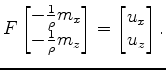
The separation operators in equations 3 and 4 are applied to the displacements fields $\left (u_x, u_z \right)$ at the receiver locations, in order to separate P-wave amplitudes from S-wave amplitudes. These operators require calculating spatial derivatives of the displacement fields in the horizontal and vertical directions. We now have omnidirectional wavefield values near the receivers, therefore applying these operators to the recreated wavefields will result in an approximation to the actual P and S-waves that were recorded by the geophones. Furthermore, the displacement separation operators in equations 6-8 can be used to separate P displacements from S displacements.

P/S separation of OBS data by inversion in a homogeneous medium