|
|
|
|
Identifying reservoir depletion patterns from production-induced deformations with applications to seismic imaging |
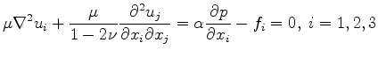
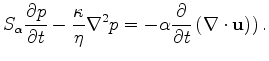
We begin by formulating a closed system of four equations that describes a homogeneous quasi-static linear poroelastic medium (Segall, 2010):
 is a spatially-distributed displacement vector field,
  is the pore pressure change,
  is a differential body-force distribution,
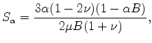
 are the shear modulus, Poisson's ratio, Biot coefficient, permeability and fluid viscosity, respectively. The storage coefficient
  is a known function of medium parameters (Segall, 2010):
 in equation 3 is Skempton's pore pressure coefficient - the ratio of induced pore pressure to the mean normal stress for undrained loading conditions. Note that the subsurface stress is absent from equations 1,2 but can be computed using the constitutive laws after these equations have been solved. Also note that the displacement and pore pressure in these equations are relative to a reference state, not the total values. The equilibrium equation 1 and flow equation 2 are fully coupled and are obtained from combining the constitutive laws for a poroelastic medium with quasi-static field equations. The equations are ``quasi-static'' in the sense that the stress field is assumed to be in a state of static equilibrium even though changes of the pore pressure in time induce changes of the stress field. We can think of this as a ``slow-change'' asymptotic approximation, both in time and space.
The most ``mathematically accurate'' way of computing the displacement field and associated pore pressure change is to solve a boundary-value problem for 1,2 with known data (e.g., known pressure evolution within existing wells, measured earth displacements or estimated stresses) used as boundary or initial conditions. However, even in the simplest cases of a homogeneous medium, analytical solutions of boundary-value problems for equations 1,2 is challenging. Uncoupling equations 1 and 2, where permissible, could result in more tractable problems, both analytically and numerically. For example, assuming a known pore pressure change, we can solve equation 1 for the displacement field  , using
 in the right-hand side as a ``body force'' distribution (Geertsma, 1973),(Segall, 1992).
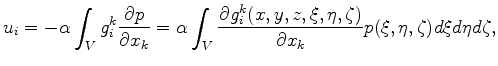
In our approach we use the elastostatic Green's tensor
 for the pure elastic equilibrium equation in the left-hand side of equation 1 to compute the displacement
as
for the pure elastic equilibrium equation in the left-hand side of equation 1 to compute the displacement
as
 (including body forces is trivial). The elastostatic tensor
in equation 4 has the meaning of the displacement along axis
(including body forces is trivial). The elastostatic tensor
in equation 4 has the meaning of the displacement along axis  at point
  due to a concentrated force along axis
  at point
 (Wang, 2000),(Segall, 2010). From equation 4 we can see that the divergence of the elastostatic tensor has the meaning of deformation due to a concentrated dilatational force.
In order to apply equation 4 to practical reservoir models and computation of surface subsidence, the corresponding Green's function should be constructed for a half-space with the free-boundary condition imposed on its bounding plane (Segall, 2010). We use the analytical expression for the Green's function obtained by Mindlin (Mindlin, 1936) - see Appendix A for the details. The integral in the right-hand side of 4 is taken over the reservoir domain and hence singularities corresponding to
 do not appear. However, the terms in non-diagonal tensor components that contain
 in the denominator blow up at locations directly above (or below) the reservoir and must be truncated in a numerical quadrature. Another important aspect of using an analytical expression for the Green's function is that the divergence in the right-hand side of equation 4 can be calculated analytically. However, in our implementation we compute the divergence using central differences of the second-order of accuracy.
|
|
|
|
Identifying reservoir depletion patterns from production-induced deformations with applications to seismic imaging |