Imaging with multiples using linearized full-wave inversion

Sigsbee2B model

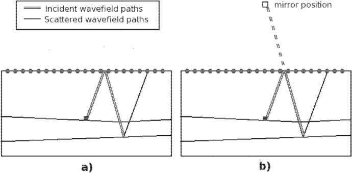
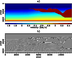
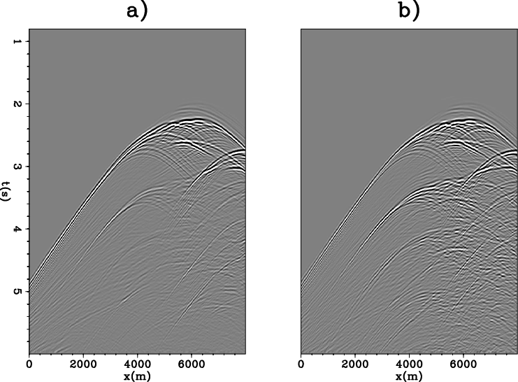
We apply LFWI to the Sigsbee2B model with the ocean-bottom geometry. Figure 7 shows the migration velocity and the reflectivity model used for this study. There are two interfaces in the migration velocity. One comes from the salt and the other comes from the basement reflector. These sharp interfaces along with the free surface boundary condition will generate the multiples. We first generate the down-going primary only data by applying the conventional mirror-imaging forward modeling operator. This is done by positioning the nodes at the mirror point across the sea-surface as shown in Figure 6. We then add 20 % of the down-going multiple energy to the down-going primary only data as shown in Figure 8. This is to simulate the case when multiple-elimination techniques cannot completely remove the multiples. We will refer to this synthetic simply as the noisy primary data. Figure 8 (b) shows the synthetic that contains first- and higher-order reflections. We will refer to this as the primary-multiple data.

mirror
Figure 6. (a) The ray-path of a mirror signal. (b) The raypath of the same signal in mirror imaging. The apparent position of the receiver is not at twicce the ocean depth above the sea bed. This assumes the sea surface is a perfect reflector. Note that the top boundary is absorbing.

panel1-m
Figure 7. (a) Migration velocity model and (b) original reflectivity model.

dataCom
Figure 8. (a) The synthetic primary (lowest-order) data with 20 % multiple energy (the noisy primary data). (b) The primary and multiples synthetic data (the primary-multiple data).

Figure 9 shows the result of applying migration and linearized inversion to the data. Panel (a) is the conventional image in which we assume a primary-only migration operator on the primary data. The red arrow indicates the artifacts in the migration image that correspond to noise included with the primary. Panel (b) is the linearized inversion result with the primary-only operator. Note the substantial improvement between migration and inversion. It has been shown (Wong et al., 2011)that linearized inversion can enhance the resolution of the image, suppress the migration artifacts, and increase the relative amplitude of true reflectors. Next, panel (c) shows the migration result achieved by applying a primary-multiple migration operator to the primary-multiple data. There are many crosstalk artifacts in this image. Without addressing the crosstalk, it is difficult to argue that panel (c) is better than panel (a). Panel (d) is the linearized full-wave inversion (LFWI) result. The annotation indicates that LFWI can properly remove the crosstalk artifacts.

In terms of convergence, since this is a classical inverse crime study, our objective function decreases to two percent of its initial value after 40 iterations.

Imaging with multiples using linearized full-wave inversion