|
|
|
|
Joint imaging with streamer and ocean bottom data |
Our synthetic study shows improvements of the joint inversion image over migrating or inverting either signal alone. There are several considerations that need to be addressed when applying these results to field data.
One consideration is related to the matching of the streamer and the OBN images, because the two surveys are acquired with different sources. Naturally, this leads to different wavelets in the data. Careful deconvolution is needed to make sure the wavelet in the image is consistent between the two surveys. Note that the two data sets are not required to have exactly the same frequency band but only the same phase (e.g., zero-phased).
Another consideration when applying this method to field data is the relative position of the reflectors between the two images.
Due to different weather conditions, the water velocity can be different between the two surveys. If the water velocity and static correction is not properly adjusted, the sea-bottom reflector between the two images might not be the same.
In addition, errors in positioning sources and receivers can also cause mismatch between the two images.
If the mismatch is not severe, one can consider applying warping in the image space (Boelle et al., 2010; Ayeni, 2011; Hale, 2011) by estimating appropriate shifts to obtain a good match.
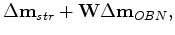
For conjugate-gradient type inversion, this simple technique requires warping when applying the migration operator:
 |
 |
 |
(4) |
|
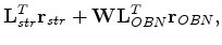 |
 is the forward warping operator that will match the OBN image update
 with the streamer image update
 .
.
 is the total image update.
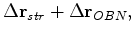
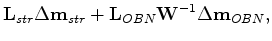
In the modeling direction, we apply unwarping before forward-modeling the gradient:
is the total image update.
In the modeling direction, we apply unwarping before forward-modeling the gradient:
 |
|
 |
(5) |
|
 |
 ,
,
 and
and
 search the total, streamer, and OBN search directions.
 is the unwarping operator.
The computational cost of linearized inversion is higher than that of migration by a factor proportional to twice the number of iterations. For OBN surveys, such additional computational cost can still be affordable. This is because the number of pre-stack calculations needed equals the number of OBN receivers in the survey. The number of migrations needed is substantially smaller than that in a towed-streamer survey. However, for towed-streamer surveys, the computational cost can be substantial. Recently, Dai et al. (2011) suggested using phase-encoding in the linearized inversion, which can reduce the computational cost substantially at the expense of introducing crosstalk into the image. In the future, we plan to combine not only the streamer and the OBN mirror signal, but to combine all 3 modes to produce one coherent image. The three modes are OBN primary, OBN mirror, and streamer data sets:
|
|
|
|
Joint imaging with streamer and ocean bottom data |
![$\displaystyle 0 \approx \left[ \begin{array}{c} \mathbf L_{str} \\ \mathbf L_{O...
...{str} \\ \mathbf d_{OBN\uparrow} \mathbf d_{OBN\downarrow} \end{array} \right].$](img34.png)