Polarity preserving decon in ``N log N'' time

Mostly causal decon

Now for the innovation. There are many pitfalls in the log domain. Seismologists are accustomed to ignoring the scale of their signals. Let the plot program figure out a suitable scale, we think. Once you take the logarithm of a signal, you are in a different world. If you double the log, you have squared the original signal. Got to be careful! What you can do safely with log signals is add or subtract something. This has the effect of scaling the original signal. Create an anticausal function $u_\tau^{\rm anti}= {\rm sgn}(\tau)u_\tau$ . The signum function ${\rm sgn}(\tau)$ is $-1$ for $\tau<0$ and $+1$ for $\tau>0$ . Adding this anticausal function to $u_\tau$ zeros the negative lags while doubling the positive lags. Because it is antisymmetric it changes the phase spectrum. It does not change the amplitude spectrum. We can use any anti-symmetrical function we wish to monkey with the phase while not changing the amplitude. We could add the antisymmetric function $u_\tau^{\rm anti}$ , but that would simply do traditional causal decon. Instead, near the origin we taper $u_\tau^{\rm anti}$ towards zero. This creates symmetric Ricker-like behavior near the origin while leaving causal behavior further away. The tapering zone used here extends beyond the Ricker width, about 20ms, but not so far as the bubble delay, about 150ms, an easy distinction. A parallel analysis is found in another paper in this report (Claerbout et al. (2012)).

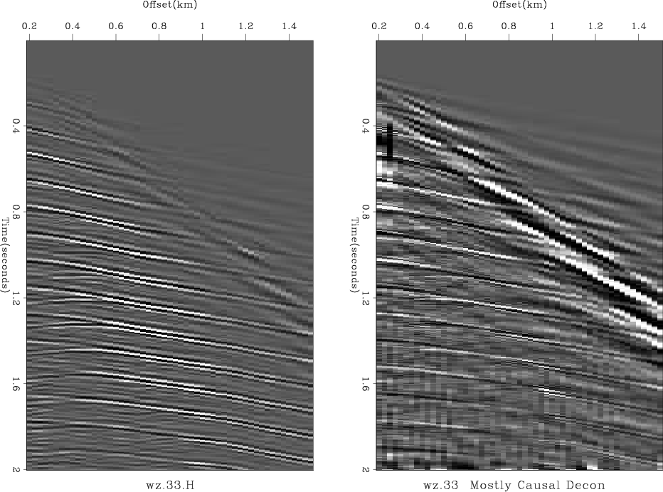
It's easy. Figures 2 and Figure 3 show the desired behavior. Hooray! The results are lovely. Better yet, they are not the end but the beginning. They are based on the simple notion that we want a white output spectrum. Our real goal is a sparse time function, not a white one. The results in these figures are simply the starting point of another paper in this report.

mostlycausal-33
Figure 2. Left is Yilmaz and Cumro shot profile 33. Right is the result of ``polarity preserving deconvolution.'' Observe enhanced visibility of alternating polarity of multiple reflections.

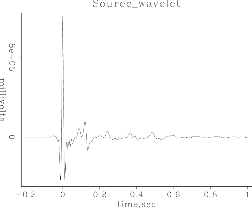
GOMwavelet
Figure 3. Shot waveform extracted from a constant offset section from the Gulf of Mexico. Peaks at zero lag as does symmetric Ricker wavelet, but for unknown reasons the peak heights are not in the (-1,2,-1) proportions of a Ricker wavelet.

Polarity preserving decon in ``N log N'' time