|
|
|
|
VTI migration velocity analysis using RTM |
We define FWI objective function as
 is the data estimated from the current model, which
is sampled from wavefield
is the data estimated from the current model, which
is sampled from wavefield  , and
, and  is the recorded data.
For the first iteration,
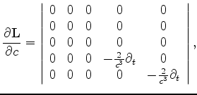
 . Therefore the first gradient
in velocity is:
. Therefore the first gradient
in velocity is:
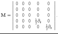
 , which is the solution of the following equation:
 , where
 .
From equation 5, we have
.
From equation 5, we have
 is chosen to make sure that
when
is chosen to make sure that
when  , equation 12 reduces to the isotropic
cross-correlation imaging condition (Claerbout, 1987).
For the purpose of velocity analysis, we often work with extended
images and generalized imaging conditions. Similarly,
we define our subsurface-offset-domain common-image gathers (SODCIGs)
, equation 12 reduces to the isotropic
cross-correlation imaging condition (Claerbout, 1987).
For the purpose of velocity analysis, we often work with extended
images and generalized imaging conditions. Similarly,
we define our subsurface-offset-domain common-image gathers (SODCIGs)
 as a column vector:
 is the half-subsurface offset, which ranges from
 to
to
 with an increment of
 .
For each element
.
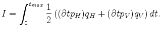
For each element  , the extended imaging condition is as follows
(Sava and Formel, 2006) :
, the extended imaging condition is as follows
(Sava and Formel, 2006) :
 is a shifting operator which shifts the wavefield
by an amount of
is a shifting operator which shifts the wavefield
by an amount of  in the
  direction. Notice that
 .
.
|
|
|
|
VTI migration velocity analysis using RTM |


![$\displaystyle {\bf I} = [I_{-{\bf h_{\rm max}}},I_{-{\bf h_{\rm max}}+\Delta {\...
...ts,I_{\bf0},\cdots,I_{{\bf h_{\rm max}}-\Delta {\bf h}},I_{\bf h_{\rm max}}]^*,$](img60.png)