|
|
|
|
VTI migration velocity analysis using RTM |
In this test, we use the same synthetic data as in the last section.
Unlike in the last example where we use the perfect velocity model,
the starting models for velocity and  are both inaccurate.
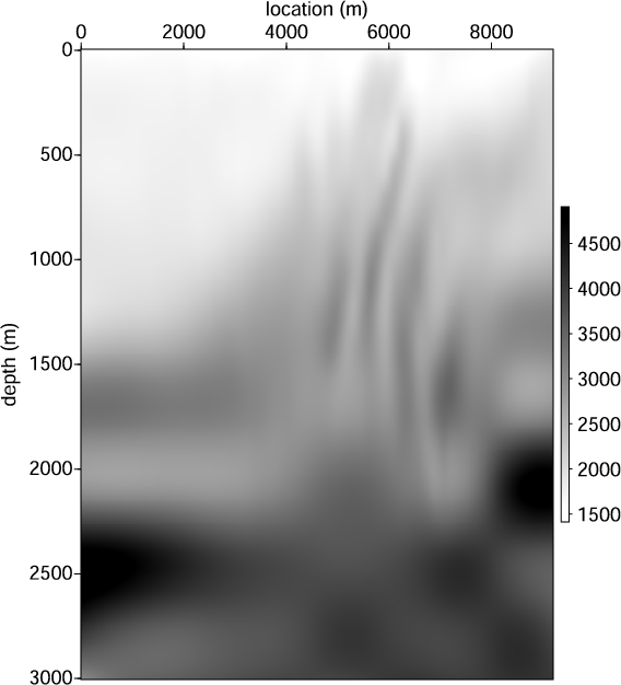
The initial velocity model and
model are shown
in Figures 7(a) and 5(a), respectively.
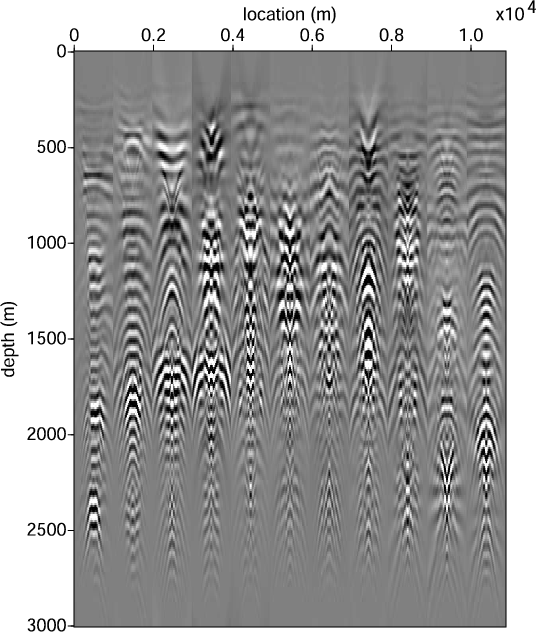
The angle gathers generated using these initial
models are shown in Figure 7(b). Significant moveout
in the angle-gather events indicates that the initial model is far
from the true model. In fact, the initial velocity has a maximum of
15% error compared with the true velocity (Figure 1(a)),
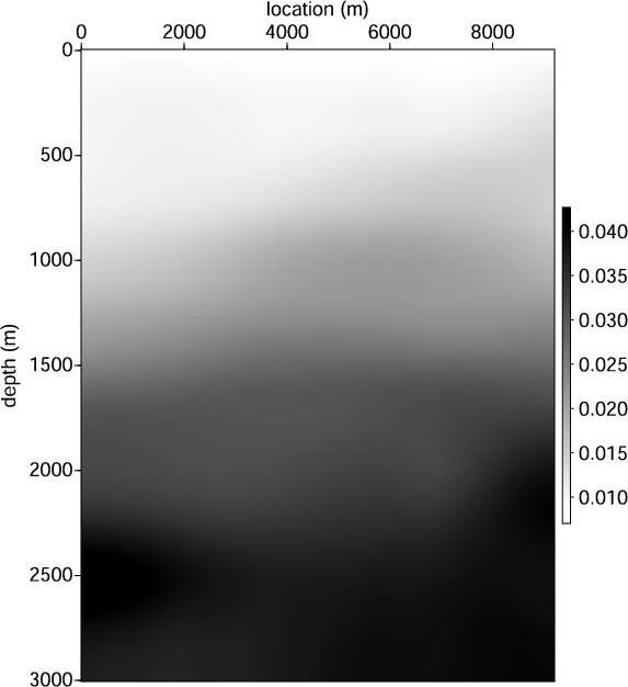
while the initial
is about 50% smaller than the true value
in the shallow part of the model. Notice
that the error in velocity has a much larger effect on the kinematics of
the seismic wave, hence a larger effect on the flatness in the angle domain.
are both inaccurate.
The initial velocity model and
model are shown
in Figures 7(a) and 5(a), respectively.
The angle gathers generated using these initial
models are shown in Figure 7(b). Significant moveout
in the angle-gather events indicates that the initial model is far
from the true model. In fact, the initial velocity has a maximum of
15% error compared with the true velocity (Figure 1(a)),
while the initial
is about 50% smaller than the true value
in the shallow part of the model. Notice
that the error in velocity has a much larger effect on the kinematics of
the seismic wave, hence a larger effect on the flatness in the angle domain.
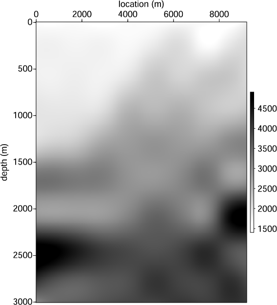
After 40 iterations, we obtain the inverted velocity and
models
as shown in Figure 8(a) and 8(b). Comparing
Figure 8(a) with Figure 1(a), we can
conclude that the inversion has successfully recovered the
high-resolution vertical structure in the shallow part of the model. Due to the
limited illumination, the steep structure in the deeper part of the model
is not well resolved. Comparing Figure 6(a) and Figure 8(b),
we notice that, because of the error in velocity, the inversion does not converge to the same solution.
This is an indication that we have not
completely resolved the ambiguity between velocity and
.
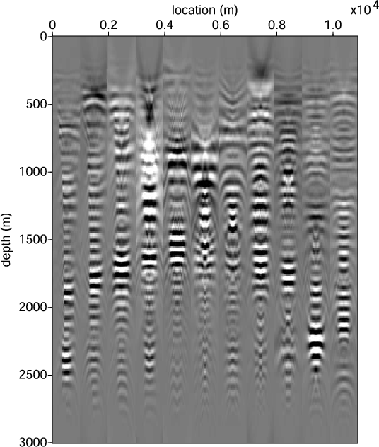
Angle gathers generated by the inverted model are shown in Figure 8(c). They are extracted from the same common-image points as in Figure 7(b). The improved model flattens the gathers across the whole section. Notice that the low-frequency energy in the water is the commonly seen wave-path energy for RTM images.
|
|---|
|
vini,angini
Figure 7. Initial velocity model (a) in m/s and the angle gathers (b) obtained using initial velocity model. Initial
model is shown in Figure 5(a).
Model error causes significant curvatures in the angle gathers. Gathers are
taken every 100 common image points from  km to
km to  km.
km.
|
|
|
|
|---|
|
vfinal,epsfinal,angfinal
Figure 8. Inverted velocity model (a) in m/s and
model (b) after 40 iterations. Angle gathers (c)
obtained by the inverted model. Angle gathers are extracted at the
same CIP as those in Figure 7(b). Improved velocity and
flattens the corresponding
angle gathers. Gathers are
taken every 100 common image points from
km to
km.
|
|
|
|
|
|
|
VTI migration velocity analysis using RTM |