Linearised inversion with GPUs

Domain decomposition

In the case where our model size exceeds that of our computing system we must break up our domain. When using Fermi GPUs the global memory is 6 Gbytes, when using Tesla GPUs we are confined to 4 Gbytes. These limited memories severely restrict models that can be allocated. For propagation we have to allocate a minimum of three 3D fields - two wavefield slices and the velocity model (the third wavefield slice can replace the first) which confines us to a symmetric model of $793$ pts$^3$ including padding regions. For RTM we need two slices for the source wavefield, two for the receiver wavefield, the velocity model, the image and the data. Assuming our time and depth axes are comparable in length, our restriction is now around $600$ pts$^3$ . 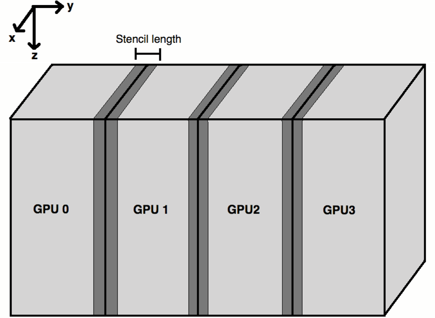We are often concerned with models more at the scale of $1000$ pts$^3$ , and for wide azimuth data sets we may have dimensions larger than this. The solution is to decompose our domain, as in Figure 4. Performance does not strongly depend on the axis over which we decide to break our domain, but for current algorithm design cutting the domain along the y axis is the most effective. We want to only cut along one dimension, rather than say break our domain into cubes along two dimensions, as this minimises the quantity of halo transfer needed (Figure 4).

domdec
Figure 4. A diagram of how to decompose the model, dark grey regions are allocated on both neighbouring GPUs

We need our sub-domains to overlap along the y-axis by half the stencil length, else information would be lost between domains. Between time steps this halo region must be transferred and then synchronised before moving to the next time step. CUDA 4.0 and above used with Fermi cards allows for Peer to Peer (P2P) GPU communication and data transfer. Previously it was necessary to explicitly route all information transfer between GPUs first through the CPU, which was significantly slower. Additionally, neighbouring GPUs can now operate on a Unified Virtual Address space (UVA), meaning there is no risk of dereferencing a pointer that has the same address on a different GPU. In fact it is now possible to dereference pointers on other GPUs or on the host, by virture of this UVA. Arrays can not span GPUs, however.

The main technique of making such a method scale linearly is by using asynchronous memory copies and kernel calls. When doing this it is possible to overlap communication with computation, hiding halo communication time. This can be done by associating certain calls to separate GPU streams, where a stream can be considered as a command pipeline. Within a stream, calls are serial, however different streams can execute concurrently. By restricting halo computation and communication to one such stream, and the other data (internal) computation to another, we can hide the halo communication. Some simplified CUDA code using streams is displayed below for reference.

for(i_gpu=0; i_gpu < n_gpus; i_gpu++){
   cudaSetDevice(i_gpu);
   kernel<<<...halo_region[],halo_stream[i_gpu]>>>(...);
   kernel<<<...internal_region[],internal_stream[i_gpu]>>>(...);
}
for(i_gpu=0; i_gpu < n_gpus; i_gpu++){
   cudaMemcpyPeerAsync(...halo_stream[i_gpu]);
}
for(i_gpu=0; i_gpu < n\_gpus; i_gpu++){
   cudaStreamSynchronise(...halo_stream[igpu]);
}
for(i_gpu=0; i_gpu < n_gpus; i_gpu++){
   cudaMemcpyPeerAsync(...halo_stream[i_gpu]);
}
for(i_gpu=0; i_gpu < n_gpus; i_gpu++){
   cudaDeviceSynchronise();
}

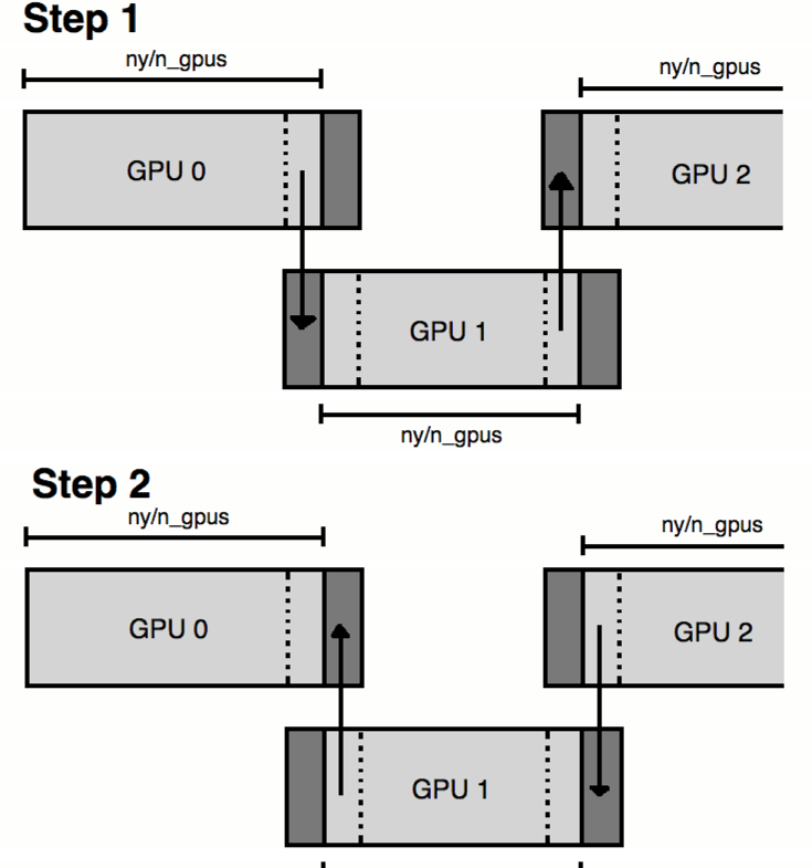
The key part to remember here is that kernel calls and async calls can overlap, providing they are defined to separate streams. So initially we loop through devices, then each one will calculate its halo region data. Once this is done, each GPU will move onto the internal data calculation. Whilst this is being calculated, each GPU moves onto the three communication loops. First off, each GPU sends its halo data to the right and receives from the left, then each device is synchronised, then each device sends to the left and receives from the right. Now each GPU has the relevant halo information for the next time step. Finally we synchronise to ensure all internal data computation is done before moving to the next time step.

halos Figure 5. A diagram of the two stages of GPU halo communication, simplified to 1D

The GPU devices are linked by PCIe switches and these switches are duplex, meaning each GPU can send and receive simultaneously - providing they are in different directions. This means a given device can send data to the GPU on its left and receive from the GPU on its right at the same time. We use the stream synchronise call because the moment a device tries to send and receive in the same direction the switch can stall, costing time. A pictorial demonstration of this is show in Figure 5.

Such a system assumes we have neighbouring GPUs on the active node in question, linked by PCIe switches. If one has GPUs on separate nodes (such as in a distributed network) MPI must be used for the halo communication. Unsurpisingly this is slower, albeit only by a factor of around 1.5x.

For acoustic propagation our internal computation time is always in far excess of halo transfer time (by an order of magnitude or so), meaning communication is always hidden and our domain decomposition scales linearly with model size, hence it is optimised. For TTI propagation this communication time approaches that of the internal data calculation, meaning for highly elastic and anisotropic media care must be taken to optimise the decomposition to ensure one is never waiting for communication. The moment we are waiting for information transfer we are not fully harnessing the potential of the GPU.

Linearised inversion with GPUs