Linearised inversion with GPUs

GPU based linearised inversion

GPU propagation augmented with random boundaries means no IO is required during propagation of either wavefield, making this a very computational effective scheme (relative to source saving.) However RTM images are often still artifact laden - low frequency artifacts can be prevalent near salt, acquisition footprints are noticeable, resolution is decreased (since we are squaring the source function) and random boundary noise may remain. All of these imperfections can be reduced by extending this scheme to least-squares inversion.

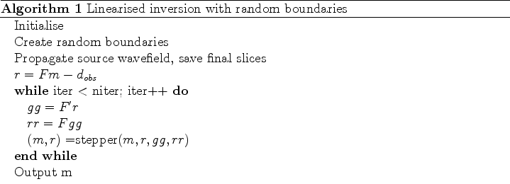
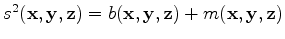
The inverse of our data modelling system can be approximated by constructing the adjoint pair of such a system and iterating in a least-squares sense. This is known as linearised inversion since we are assuming we know the kinematic model (the background velocity) and are trying to retrieve the high frequency (perturbation) part of the Earth model. This amounts to describing our slowness function as $s^2(\mathbf{x,y,z}) = b(\mathbf{x,y,z}) + m(\mathbf{x,y,z})$ . As an algorithm it can be described by Algorithm 1. Here $F$ is our operator, $F'$ its adjoint, $r$ the data-space residual, $m$ the current model estimate, $d_{obs}$ the input data, $gg$ the gradient and $rr$ the back-projected residual. The stepper then updates the current model estimate and data-space residual. Since we are not changing our boundaries between iterations, we first forward our source wavefields and save the final slices necessary for back propagation. These can then be back propagated along with the receiver wavefield in the $gg = F' r$ step of the algorithm.

The adjoint process, $F'$ , is identical to the aforementioned RTM scheme with random boundaries. Now we must try and implement the forward process, $F$ , in the most computationally efficient way. Initially we must think about our stencil. To take the spatial derivative of the wavefield we convolve the data with a star-shaped stencil, for an 8th order scheme in 3D this stencil is 25 points in total, as each direction shares the centre value. Previously we only needed to define the velocity value at the centre of our stencil, as the forward procedure was spraying the information to neighbouring grid cells. The adjoint of this propagation requires velocity values to be defined along the entirety of the stencil, as we now need the information from all points being calculated to carry to all new points. This means that in addition to allocating our wavefield values in the GPU kernel, we must also allocate the same number of velocity points.

Previously we were using texture memory to store our velocity values to take advantage of caching and automatic boundary control features (Leader and Clapp, 2011). What we can now do is save the relevant velocity values to shared memory, taking care that we do not saturate the memory. For large stencil sizes this can require the use of smaller blocks. By defining our local velocity array in the same way that we do our wavefield values, we can still take advantage of shared memory. This extra memory allocation and computation causes this adjoint propagator to be about 81% the speed of forward propagation. By only using texture memory we see this drop to around 43%, and by using global memory this decreases to 38%. On a Tesla GPU this final speed would be slower again, since Fermi cards provide some global L1 and L2 cache options. In order to make the system fully adjoint the source wavefield must be propagated through the same random boundary as in the corresponding RTM, but we can damp the data wavefield. Since we are now using equation 1 we have no time reversal problems, because the sense of time for both the source wavefield and the data wavefield are the same.

The stepper is performed on the CPU. The reasons for this are twofold - firstly we want to transfer our data and image back to the CPU for writing purposes, so doing the model update on the CPU creates no unnecessary data transfer. Additionally, our solver is just a series of vector operations (dot products and subtractions) and such operations can not be accelerated by the GPU. They no longer have a SIMD corollary and global memory operations on the CPU are faster than on the GPU, often by a factor of 2 or 3.

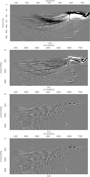
Results from this linearised inverse scheme can be seen in Figure 3, in which we are attempting to recover the reflectivity model shown in Figure 2. Here we have 60 inline shots at a spacing of 100m and two crossline shots at a spacing of 1km, receivers are in a dense 825x200 grid. We can clearly see the inverse scheme improving the resolution of the top of the salt and mitigating the associated low-frequency artefacts.

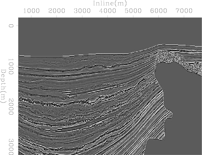
srfl Figure 2. A 2D slice from the reflectivity model that we are attempting to recover.

imgc
Figure 3. RTM and linearised inversion example 2D slices. (a) shows the raw RTM result, (b) raw inversion after 5 iterations, (c) RTM with lowcut bandpass filter and (d) inversion after 5 iterations and lowcut filter.

Linearised inversion with GPUs