|
|
|
|
Image gather reconstruction using StOMP |
For the correlation gather construction problem, I attempted to
encode multiple different correlations into each data sample. In terms
of operators, we can think of the subsampling of correlations as applying
a subsampling operator  to all possible correlations
  . In the
phase encoded case, we are going to add another operator
. In the
phase encoded case, we are going to add another operator  that first
sums a number of different correlations together and then subsamples
them leaving a new dataset
that first
sums a number of different correlations together and then subsamples
them leaving a new dataset
 .
This in turn changes the operator
.
This in turn changes the operator  in algorithm 1
to
in algorithm 1
to
 . For this test, I combined 20 different correlations
in a random pattern to form each data point.
Figure 8 shows the same three offset and angle
gathers seen in Figures 4 and 6. Note
the noticeably better job recovering the deeper
portion of subsurface offsets. Figure 9 shows
the angle gathers from the fully sampled correlation gathers and
the subsampled, phase encoded gathers muted to the believable
angle range. The gathers with the notable
exception of more lower frequency noise in the recovered gathers.
. For this test, I combined 20 different correlations
in a random pattern to form each data point.
Figure 8 shows the same three offset and angle
gathers seen in Figures 4 and 6. Note
the noticeably better job recovering the deeper
portion of subsurface offsets. Figure 9 shows
the angle gathers from the fully sampled correlation gathers and
the subsampled, phase encoded gathers muted to the believable
angle range. The gathers with the notable
exception of more lower frequency noise in the recovered gathers.

|
|---|
|
data-2
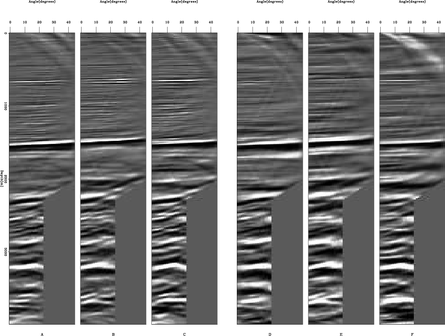
Figure 8. A, B, and C show the recovered subsurface offset gathers using compressive sensing as shown in plot A, B and C of Figure 4 and 6. D, E, and F show the corresponding angle gathers. Note the noticeable improvement in A, B, and C compared to the data shown in Figure 6. |
|
|
|
|---|
|
compare
Figure 9. A comparison of the angle gathers after muting of the fully sampled correlation gathers (A, B, and C) and the phase encoded, subsampled correlation gathers (D, E, and F). |
|
|
|
|
|
|
Image gather reconstruction using StOMP |