 |
 |
 |
 | Image gather reconstruction using StOMP |  |
![[pdf]](icons/pdf.png) |
Next: StOMP algorithm
Up: Clapp: Compressive sensing
Previous: Image gathers and wavelet
Compressive sensing is a statistical technique attributed to
Donoho (2006),
but whose start could be placed as early as the basic pursuit work of
Mallat and Zhang (1993). A compressive
sensing problem at its heart is a special case of a missing data problem. In geophysics, we often
think of a missing data problem as solving for a model  given some data
  which
exist
in the same vector space. We have a masking operator
which
exist
in the same vector space. We have a masking operator  (1 where the data is known, 0 elsewhere). We add
in some knowledge of the covariance of the model through a regularization operator
(1 where the data is known, 0 elsewhere). We add
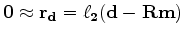
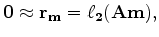
in some knowledge of the covariance of the model through a regularization operator  . We then estimate the
best model from
the following system of equations in a
. We then estimate the
best model from
the following system of equations in a  sense,
 |
|
|
|
 |
|
|
(3) |
where  and
and  are the result of taking the
norm
of the first and second equations.
The success of this approach relies on the accuracy of
to describe the covariance of the model.
are the result of taking the
norm
of the first and second equations.
The success of this approach relies on the accuracy of
to describe the covariance of the model.
Compressive sensing approaches the problem from a different perspective. It starts from the notion that
there exists a basis function that
can be transformed into through the
linear operator  in which very few non-zero
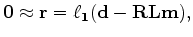
elements are needed to represent the signal. The compressive sensing approach is then to set up the missing data problem
in two phases. First, estimate the elements of the sparse basis function
through,
in which very few non-zero
elements are needed to represent the signal. The compressive sensing approach is then to set up the missing data problem
in two phases. First, estimate the elements of the sparse basis function
through,
 |
(4) |
where we are now estimating
in the  sense. We can then apply
  to recover the full model.
The magic of compressive sensing is that you only need to collect a small multiple, typically
4-5, more data points than the number of non-zero basis elements. In the case of correlation gather compression
this would indicate collecting in the range of 5% of the correlations should be
sufficient to recover the entire model, much smaller than
what the Nyquist-Shannon (Nyquist, 1928) criteria would suggest.
to recover the full model.
The magic of compressive sensing is that you only need to collect a small multiple, typically
4-5, more data points than the number of non-zero basis elements. In the case of correlation gather compression
this would indicate collecting in the range of 5% of the correlations should be
sufficient to recover the entire model, much smaller than
what the Nyquist-Shannon (Nyquist, 1928) criteria would suggest.
|
|
|
|
| Image gather reconstruction using StOMP | |
|
Next: StOMP algorithm
Up: Clapp: Compressive sensing
Previous: Image gathers and wavelet
2012-05-10