Tomographic full waveform inversion (TFWI) by combining full waveform inversion with wave-equation migration velocity analysis

Marmousi model

To test the convergence and resolution characteristics of the TFWI method, we applied it to the inversion of a synthetic data set generated assuming the modified Marmousi model shown in Figure 9. This model is the classical Marmousi with the addition of a 500 m water layer. The data were modeled assuming 93 shots with 100 m spacing and a Ricker wavelet with fundamental frequency of 15 Hz. The reflected wavefields were recorded by 461 receivers with fixed spread and 20 m spacing.

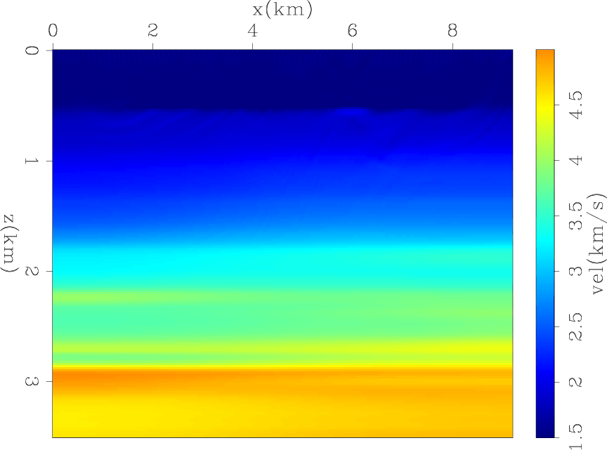
We compare the results of three inversion methods starting from the model shown in Figure 10, which was obtained by applying strong horizontal smoothing to the true model. Figure 11 shows the model obtained with conventional FWI; that is, by minimizing the objective function expressed in equation 1. As expected, conventional FWI fails because of its well-known difficulties with global convergence. The resulting model is almost identical to the starting one, with only a few shallow velocity discontinuities being imaged.

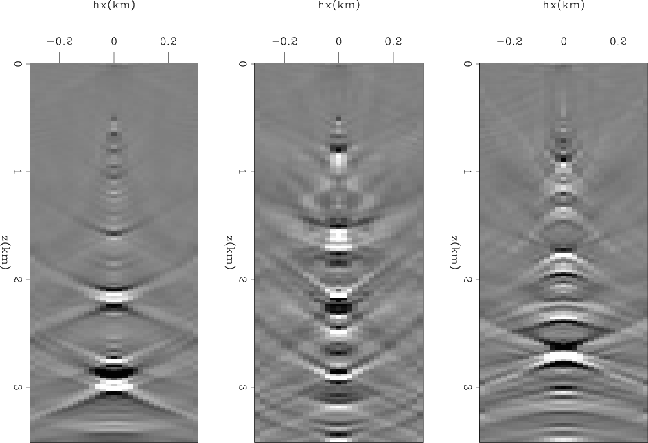
Figure 12 and 15 show the results of extended FWI (EFWI); that is, the minimization of the objective function expressed in equation 5. Figure 12 shows the zero subsurface offset section, displayed in color to facilitate the analysis of the long-wavelength components of the velocity. These components are similar in the final model and in the initial model. However, in contrast with the simple FWI, reflectivity is now imaged across the section, though misplaced and only partially focused because of the persistent errors in the long-wavelength components of the velocity. Figure 15 shows three sections of the difference cube obtained by subtracting the starting model from the final model. These sections are taken at fixed horizontal coordinates and are functions of depth and subsurface offset. These images are analogous to migration subsurface-offset common image gathers; they show the lack of focusing of the model along the subsurface-offset axis.

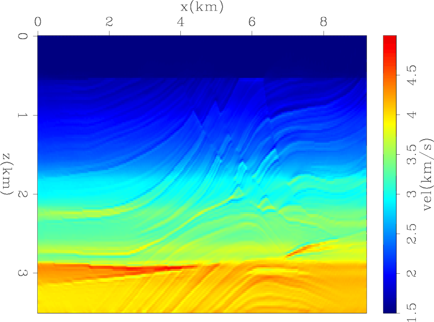
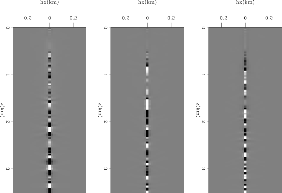
Figure 13 and 16 show the results of the proposed tomographic full waveform inversion (TFWI). To compute these results we minimized an objective function defined by the sum of equation 5 and equation 6. The zero subsurface-offset section (Figure 13) shows remarkable convergence towards the true model, in particular in the middle of the section where the model is well illuminated by the modeled data. The offset-domain common image gathers shown in Figure 16 confirm that the final model correctly focuses the reflected events. Similarly to the previous example (Gaussian anomaly), the gathers shown in Figure 16 appear artificially focused around zero subsurface offset. As discussed previously, this appearance is caused by the DSO term in the objective function forcing the focusing of the image even beyond what would have been the focusing with the true model.

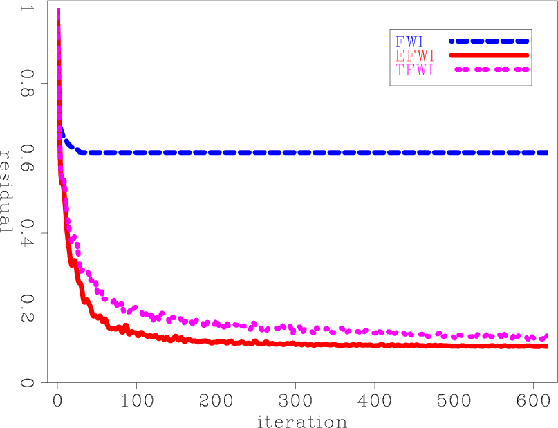
Finally, Figure 14 shows normalized values of the norm of the data residuals as a function of iterations for all three methods we discussed: FWI in blue, EFWI (i.e. minimizing only objective function 5) in red and TFWI (i.e. minimizing sum of objective functions 5 and 6) in magenta. Notice that in the case of TFWI, even if the objective function had two terms, only the value of $J_{\rm EFWI}$ (i.e. the data fitting term) is plotted in the graph. The graphs show that FWI has not converged even after hundreds of iterations. The data residuals decrease more quickly for EFWI than for TFWI because EFWI does not need substantial changes in the long-wavelength components of the model to fit the data. However, the magnitude of the final residuals is comparable between the two methods.

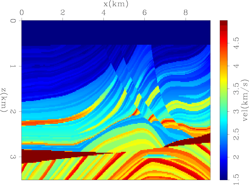
seg1-vtrue Figure 9. Modified Marmousi model used for numerical tests.

seg1-init Figure 10. Starting model for inversions.

seg1-inv0 Figure 11. Final model when minimizing objective function 1 (FWI).

seg1-inv1 Figure 12. Final model when minimizing objective function 5 (EFWI).

seg1-inv2 Figure 13. Final model when minimizing sum of objective functions 5 and 6 (TFWI).

seg1-inv-all-fixed Figure 14. Graphs of data residuals as function of iterations for: FWI (blue), EFWI (red), and TFWI (magenta).

seg1-inv1-dv1 Figure 15. Final model subtracted from initial model taken at x=2.5, 5, and 7.5 km for EFWI.

seg1-inv2-dv1 Figure 16. Final model subtracted from initial model taken at x=2.5, 5, and 7.5 km for TFWI.

Tomographic full waveform inversion (TFWI) by combining full waveform inversion with wave-equation migration velocity analysis