Tomographic full waveform inversion (TFWI) by combining full waveform inversion with wave-equation migration velocity analysis

Gaussian Anomaly

To illustrate the interplay between different scales of the velocity during the inversion we applied the proposed method to a two-layer model with a Gaussian anomaly in the middle of the first layer, as shown in Figure 1. The velocity of the top layer is 3 km/s and of the bottom layer is 3.5 km/s. The velocity at the center of the Gaussian anomaly is 3.5 km/s. The interface between the layers is at 2 km depth and the Gaussian anomaly is centered at 1 km depth.

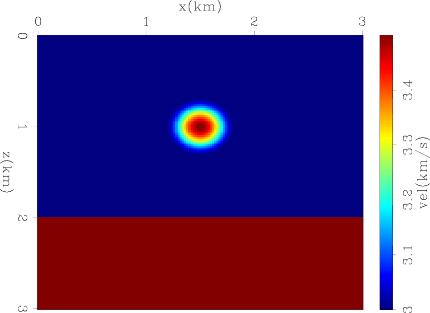
A Ricker wavelet with a fundamental frequency of 15 Hz and temporal sampling of 1.5 ms was used as a source function to model the data. The wavefields were generated by 31 sources with a spacing of 100 m and recorded by 151 fixed receivers with a spacing of 20 m. The maximum offset is 1.5 km. The initial model is a constant model of 3 km/s velocity.

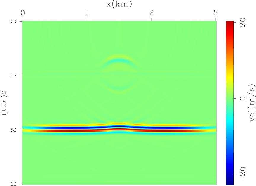
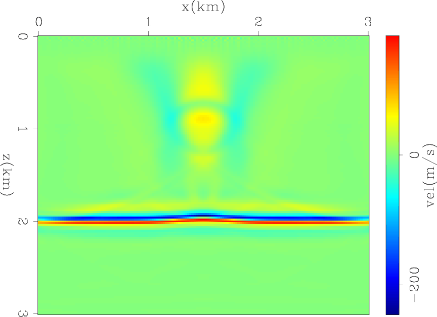
Figure 2 shows the difference between the velocity model estimated after one iteration and the starting model. As expected, the reflector is well imaged, though not perfectly focused under the velocity anomaly. Figure 3 shows a rescaled window of Figure 2 around the anomaly. It shows how the reflections from the anomaly measured from the low-frequency components of the data start outlining the contour of the anomaly. Figure 4 shows the difference between the initial and the inverted model after 2000 iterations. Figure 5 shows a rescaled window of Figure 4 around the anomaly. The anomaly is now fairly well focused. However, the maximum amplitude of the estimated anomaly is still a fraction of the amplitude of the true anomaly, but better recovered than if it had been estimated using conventional velocity estimation methods based only on the transmission effects (Almomin and Biondi, 2012).

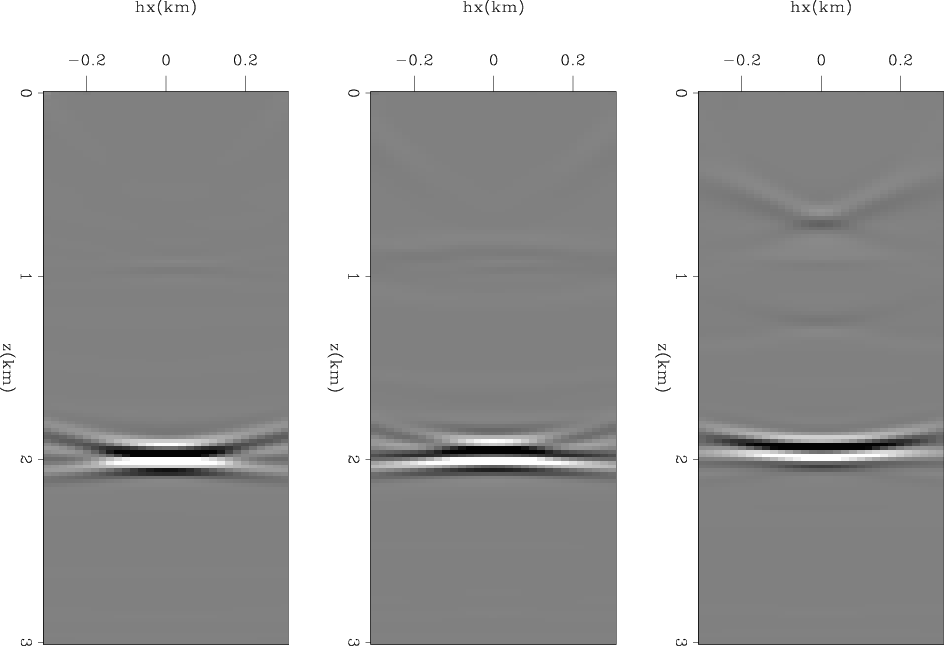
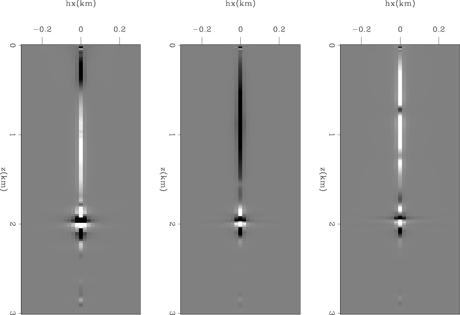
Figure 6 shows three sections of the difference cube obtained by subtracting the starting model from the model obtained after one iteration. These sections are taken at fixed horizontal coordinates and are functions of depth and subsurface offset. These images are analogous to migration subsurface-offset common image gathers; they show the lack of focusing of the model along the subsurface-offset axis. Figure 7 shows the gathers taken at the same locations as the ones shown in Figure 6, but after 2000 iterations. The gathers are now well focused around the zero-offset axis, indicating that the final model well explains the kinematic effects of the reflections that propagated through the velocity anomaly. Indeed, the gathers shown in Figure 7 appear artificially focused around zero subsurface offset. This appearance is caused by the DSO term in the objective function forcing the focusing of the image even beyond what would have been the focusing with the true model. In the data domain this ``extra'' focusing causes extrapolation of events beyond the recorded offsets (Clapp, 2005).

Figure 8 shows the normalized data residual as a function of iterations. The residual has not completely not flatten out and converged to zero; further iterations would improve the results.

seg1-gauss-true Figure 1. The true velocity model.

seg1-gauss-iter1 Figure 2. The difference between inverted and initial model after one iteration.

seg1-gauss-iter1-top Figure 3. Zoom of the difference between inverted and initial model after one iteration. Notice the slight vertical stretch with respect to Figure 2.

seg1-gauss-inv Figure 4. The difference between inverted and initial model after 2000 iterations.

seg1-gauss-inv-top Figure 5. Zoom of the difference between inverted and initial model after 2000 iterations. Notice the slight vertical stretch with respect to Figure 4.

seg1-gauss-iter1-dv1 Figure 6. The difference between inverted and initial model after one iteration. These sections were taken at x=.09, 1.2, and 1.5 km.

seg1-gauss-inv-dv1 Figure 7. The difference between inverted and initial model after 2000 iterations. These sections were taken at x=.09, 1.2, and 1.5 km. Compare with Figure 6.

seg1-gauss-res Figure 8. The normalized residual as a function of the number of iterations.

Tomographic full waveform inversion (TFWI) by combining full waveform inversion with wave-equation migration velocity analysis