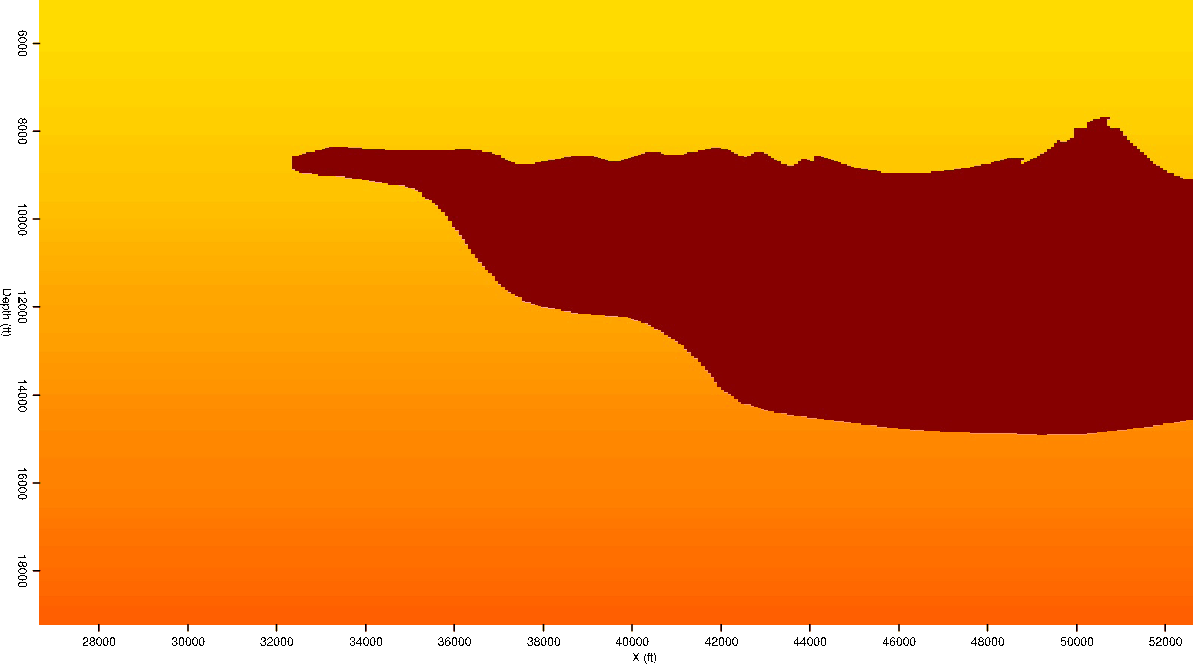
Fast velocity model evaluation with synthesized wavefields

Synthetic example

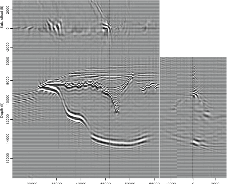
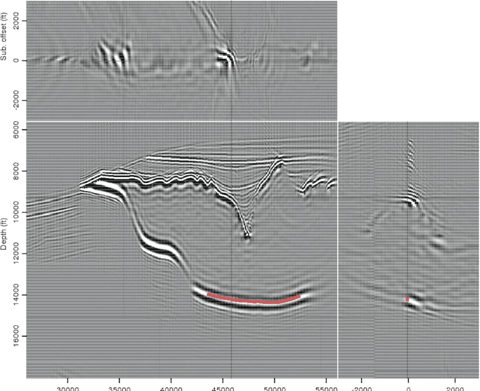
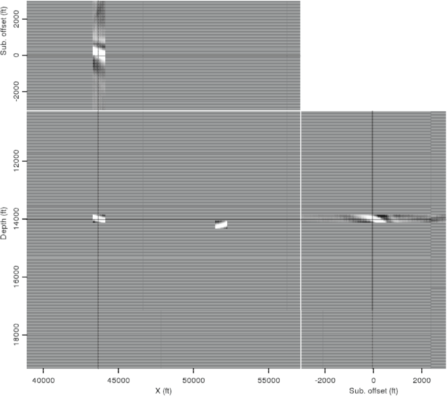
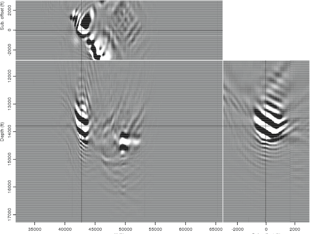
The above procedure will now be demonstrated using two different initial images derived from the Sigsbee synthetic model. Figure 1(a) is a perfect-velocity, full migration of the Sigsbee data, which will be used for the first example. Figure 1(b) shows a manually-picked reflector chosen for further analysis; in this case, the base salt has been chosen because it should be particularly sensitive to different interpretations of the salt body's shape and velocity, the two model variations that will be tested. Finally, Figure 2 shows two image locations isolated from the selected reflector. Note that most of the energy is focused near zero subsurface-offset, since the true velocity model was used for the initial image.

img-act,picks
Figure 1. (a) A true velocity image using data from a section of the Sigsbee synthetic model; and (b) a base-of-salt reflector selected for further analysis because of its sensitivity to changes in the salt interpretation.

act-pts Figure 2. Isolated image locations selected from the reflector picked in Figure 1(b).

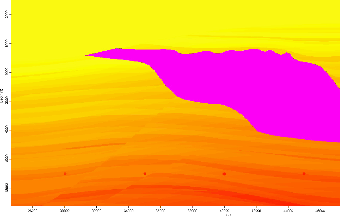
After synthesizing the source and receiver wavefields as described in the previous section, the new wavefields were imaged using three different velocity models. First, the true model, seen in Figure 3(a). Second, an alternative model created via automatic image segmentation, in which an interpreter has chosen to include an extra chunk of salt (Figure 3(b)). The third model tested was identical to the true model in salt shape, but with a salt velocity 5% slower than the true model.

zvel-act,zvel-filled
Figure 3. Two different velocity models to be tested. The model in (a) is the true Sigsbee model, while (b) is an alternate model created by one possible automatic segmentation of the initial image.

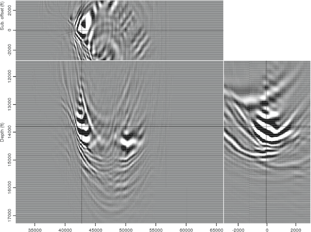
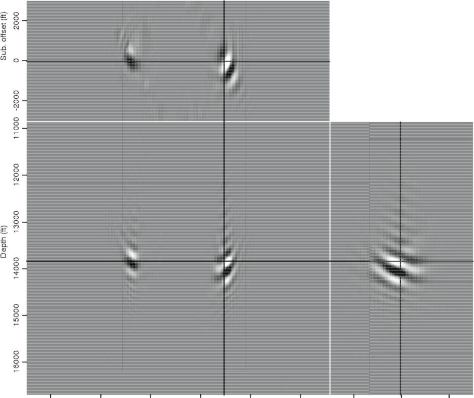
Resulting images from the Born-modeled data are seen in Figure 4. Panel 4(b), the result of migrating with the extra-salt model in Figure 3(b), is clearly the least well-focused image. However, it is difficult to qualitatively distinguish between the other two results. Table 1 gives the results of calculating the $F$ value from equation 5 for each of the images. As expected, the result using the true model has a higher $F$ value, indicating it is more well-focused.

born-act,born-af,born-as
Figure 4. Three images of the Born-modeled data using three different migration velocity models: (a) the true model; (b) the extra-salt model; and (c) the slow-salt model. In this example, the initial image was created with the true model.

Table 1: Calculations from equation 5 for each migration velocity model, after the initial image and synthesized wavefields were created using the true velocity model.

Migration model	$F$ value
True velocity	0.883
Extra salt	0.879
Slow salt	0.864

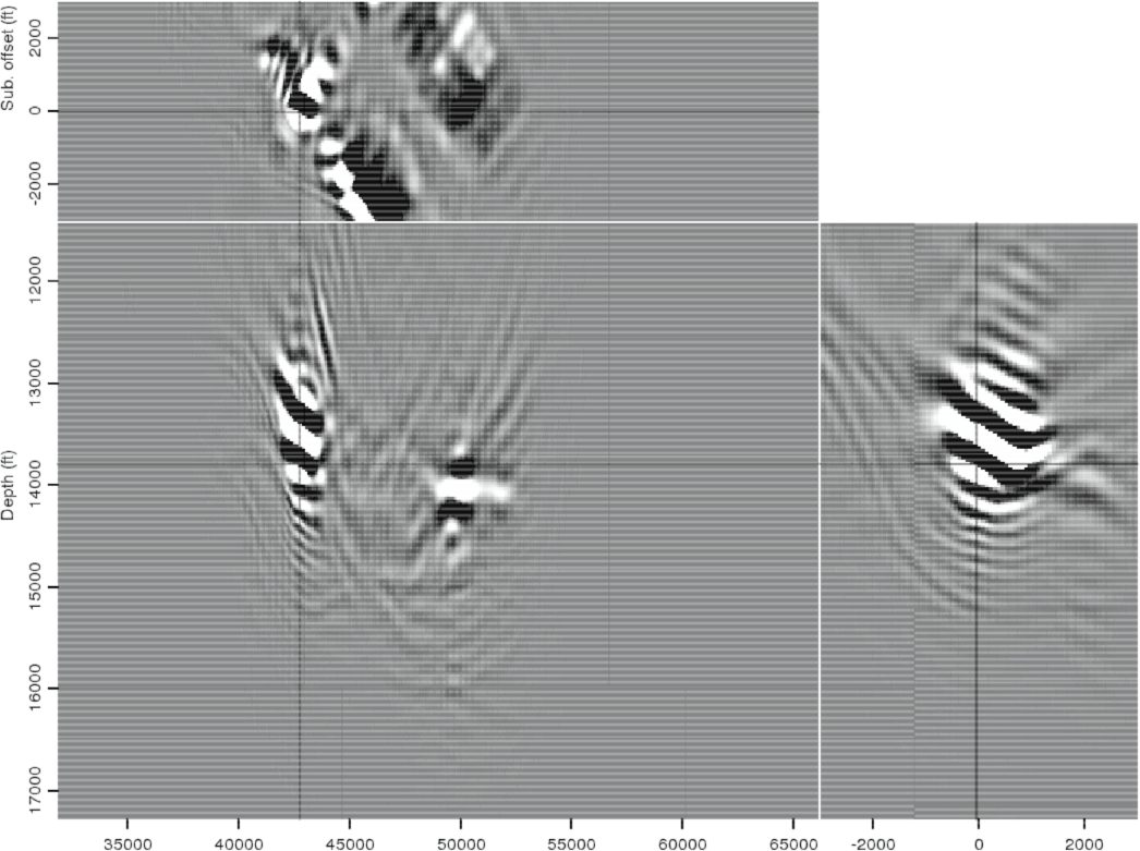
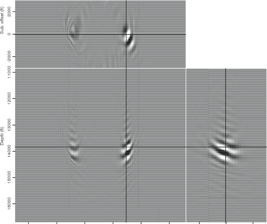
The second example uses an initial image created with an incorrect velocity model; in this case, the ``slow salt" model described above. The results corresponding to each velocity model can be seen in Figure 5. Again, the extra-salt model is clearly inferior, but the differences between the other two results are more subtle. The $F$ -value calculations in Table 2 confirm that the true model yields the optimal result, even though the slow-salt model was used to create the initial image and both synthesized datasets. In both examples, the differences between the calculated $F$ values are relatively small; further investigation should determine how confidently such differences may be interpreted, especially when working with noisier field data.

born-sa,born-sf,born-ss
Figure 5. Three images of the Born-modeled data using three different migration velocity models: (a) the true model; (b) the extra-salt model; and (c) the slow-salt model. In this example, the initial image was created with the slow-salt model.

Table 2: Calculations from equation 5 for each migration velocity model, after the initial image and synthesized wavefields were created using the ``slow salt" velocity model.

Migration model	$F$ value
True velocity	0.621
Extra salt	0.561
Slow salt	0.613

Fast velocity model evaluation with synthesized wavefields