Preconditioning a non-linear problem and its application to bidirectional deconvolution

PEF versus GALI-PEF preconditioning

In this subsection, we test the PEF preconditioning and GALI-PEF preconditioning on bidirectional deconvolution. Fu et al. (2011) shows that the method proposed by Claerbout et al. (2011) produces the most stable result among the three bidirectional deconvolution methods considered above. Therefore, we use Claerbout et al. (2011) to compare these two preconditionings to make the comparison reliable.

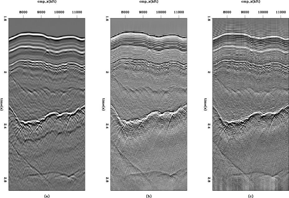
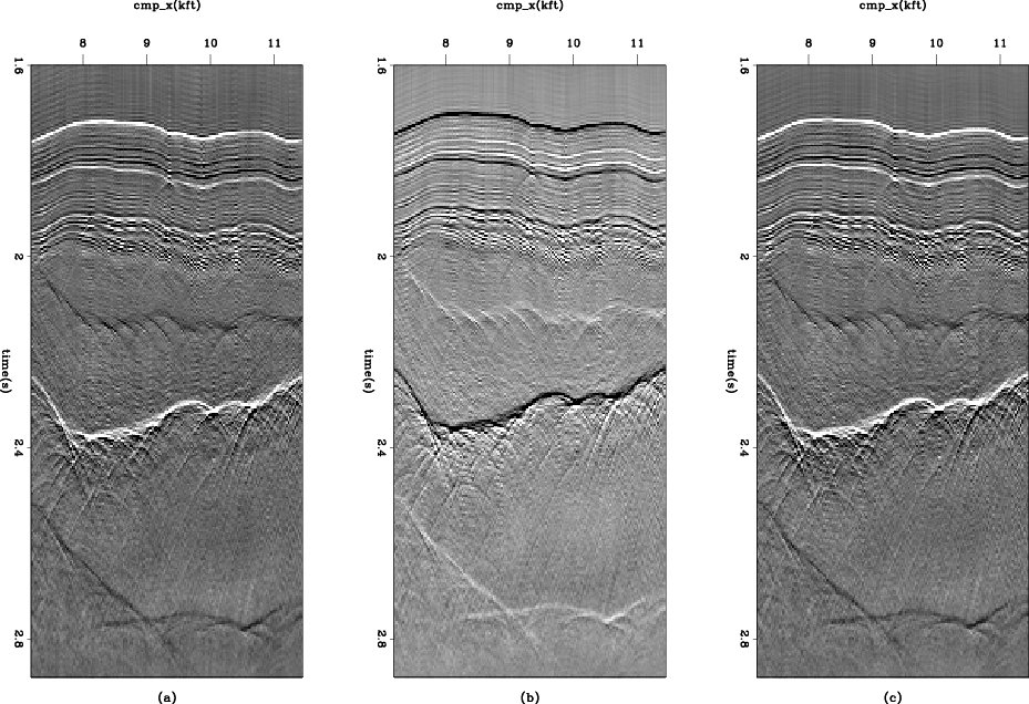
We use the same field data shown in the previous subsection for this example. First, we convolve the data with PEF and GALI-PEF preconditioning respectively, as shown in Figure 10. Then we apply bidirectional deconvolution to the convolution results, as is displayed in Figure 11. We may draw the following conclusions from the comparison results.

GALI-PEF preconditioning helps constrain the spike to the central wavelet. As the data shows, the events in Figure 7 look like a Ricker wavelet, with two weak side lobes and one strong middle lobe. We expect the preconditioned spike to coincide with the strong middle lobe. Because PEF is a causal filter with causal inverse, it shifts the output toward the first lobe of the Ricker wavelet. Thus the polarity of the output is the same as the first lobe of the Ricker. From panel (b) in Figure 10, the strong event(the water bottom) is black. This polarity, as well as its output location, is the same as that of the first lobe of the mixed-phase wavelet, around 1.8 seconds in Figure 10. Focusing on the first lobe in preconditioning leads to same effect in the bidirectional deconvolution. Panel (b) in Figure 11 shows exactly the same outcome: the output is in the same location and has the same polarity as the first lobe of the Ricker wavelet.

On the other hand, GALI-PEF preconditioning helps shift the time of output. Panel (c) in Figure 10 shows that the event is produced in the same location and polarity as the middle of the Ricker wavelet. The same is true of the bidirectional deconvolution results. To take the water bottom for example, the event appears white in both GALI-PEF preconditioning and its bidirectional deconvolution result, which is the same polarity as the middle lobe of the wavelet. This centered spike is the usual goal of GALI-PEF preconditioning, but by manipulating the length of the gap, we can shift the spike to any desired location. In this case, the gap between the first ghost and first arrival is roughly 10-15 ms. If the gap in GALI-PEF preconditioning is longer than this separation, the output will move towards the second side lobe of the wavelet, and vice versa.

Unfortunately, however, GALI-PEF preconditioning does not improve the result compared to PEF preconditioning. Both the PEF and GALI-PEF preconditioning results are almost the same except for reversed polarity and a time shift. In addition, the precursors in Figure 10(c) are strong, because of the anti-causal integration. From another perspective, although the GALI-PEF preconditioner produces a noisier, more resonant section than does PEF, that section illustrates the polarity more clearly than does PEF. Also, the interval between every two adjacent precursors illustrates the gap between first ghost and first arrival.

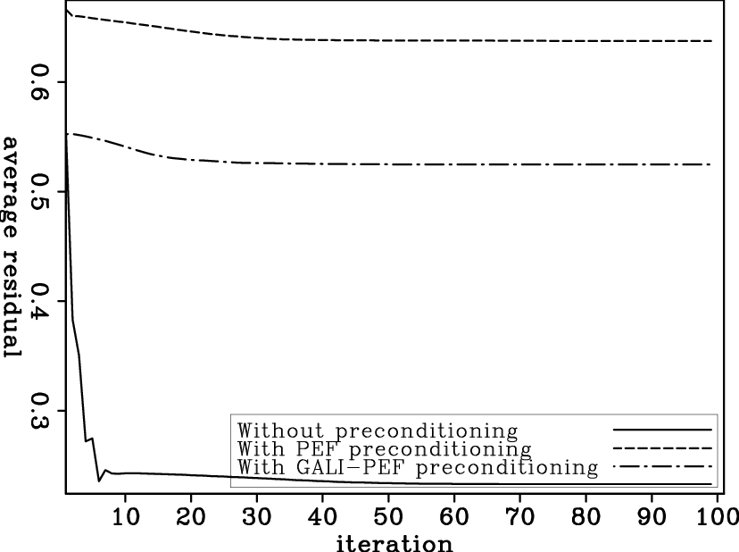
Both preconditioning methods speed convergence. The convergence rates with and without preconditioning are shown in Figure 12. The average mismatch here is measured by using a hybrid penalty function (Claerbout, 2010):

$$\frac{{\bar r}} {R} = r(\bar H) = \sqrt {(\frac{1} {N}\sum\limits_{i = 1}^N {\sqrt {1 + \frac{{r_i^2 }} {{R^2 }}} } )^2 - 1}$$ (11)

where $H(r) = \sqrt {R^2 + r^2 } - R$ , and $R$ is the threshold. This expression of the misfit is dimensionless and reflects the speed of convergence. Note that the three convergence curves in Figure 12 originate from different points, because the average residual without preconditioning is calculated directly from the raw data, whereas the ones with the two preconditioning methods are calculated from the data transformed by PEF and GALI-PEF preconditionings respectively. Thus, we only consider the relative trend, not the absolute value, of the curves. We notice that the convergence rates drop somewhat with preconditioning, because both PEF and GALI-PEF already help reduce the average mismatch. However, convergence is reached soon after 30 iterations with the help of preconditioning, whereas without preconditioning convergence takes more than 55 iterations. Therefore, preconditioning does reduce the computational cost.

Both methods of preconditioning improve bidirectional deconvolution. The logarithm bidirectional deconvolution proposed by Claerbout et al. (2011), which estimates the filters in the Fourier domain, is more stable than the one proposed by Shen et al. (2011). Thus the result depends less on preconditioning in the logarithm method. However, we still notice that both methods of preconditioning improve the results by reducing precursors. In addition, the unknown event around 2.4 seconds in panel (a) of Figure 11 becomes weaker in the results with preconditioning, especially in bidirectional deconvolution with PEF preconditioning.

dataside
Figure 10. Given the common offset data in Figure 7, (a) 1/3 of original data; (b) data transformed by PEF preconditioning; (c) data transformed by GALI-PEF preconditioning. These three panels are the inputs to the bidirectional deconvolution output in Figure 11.

modelside
Figure 11. Given the common offset data in Figure 7, (a)bidirectional deconvolution without preconditioning; (b) bidirectional deconvolution with PEF preconditioning (c) bidirectional deconvolution with GALI-PEF preconditioning.

resavg Figure 12. Convergence rate of the results in Figure 11. Both preconditioning methods speed convergence.

Preconditioning a non-linear problem and its application to bidirectional deconvolution