Preconditioning a non-linear problem and its application to bidirectional deconvolution

Bidirectional deconvolution with and without preconditioning

We considered three bidirectional deconvolution methods (Zhang and Claerbout (2010), Shen et al. (2011) and Claerbout et al. (2011)). Of these three methods, the method proposed by Shen et al. (2011) most needs preconditioning. We therefore test our preconditioning on this method to illustrate the effectiveness and limitation of preconditioning.

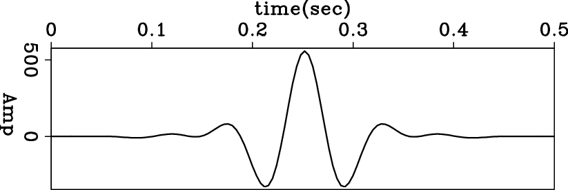
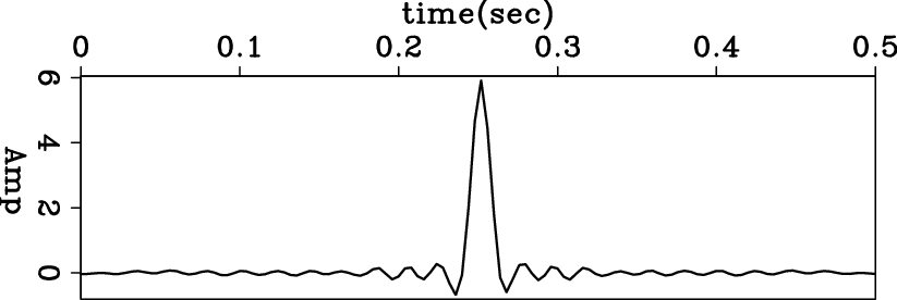
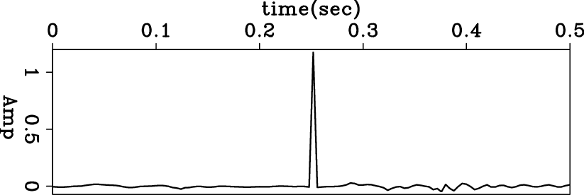
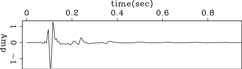
To illustrate the capabilities of preconditioning, we analyze the results obtained by inverting a zero-phase wavelet. This wavelet is created by convolving the minimum-phase with its own time-reversed wavelet. Figures 2, 3 and 4 show the zero-phase wavelet and its bidirectional deconvolution proposed by Shen et al. (2011), without and with PEF preconditioning. The results show that the wavelet is not completely compressed into a spike without preconditioning, but preconditioning does yield a spike. These results indicate that preconditioning steers the non-linear problem away from unwelcome local minima. However, we can still see slight ringing around the spike in the preconditioned result, indicating that PEF preconditioning does not fully guide the result to the global minimum. This suggests we should introduce more prior knowledge into the preconditioning.

data2 Figure 2. Zero-phase wavelet as the input to the bidirectional deconvolution in Figure 3 and 4.

mod2new Figure 3. Deconvolution result without preconditioning. The wavelet is not completely compressed into a spike.

mod2newpre Figure 4. Deconvolution result with PEF preconditioning. The wavelet is compressed into a spike.

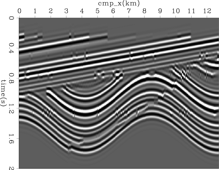
After deconvolving the simple 1D case, we test preconditioning on more complicated 2D synthetic data. Figure 5(a) shows the starting reflectivity model. Figure 5(b) shows the data generated by convolving the reflectivity model with the zero-phase wavelet in the previous section. All traces in the data share the same wavelet during modeling and deconvolution.

syn3,data3
Figure 5. (a) The 2D synthetic reflectivity model; (b) the synthetic data generated using the zero-phase wavelet.

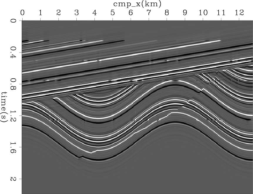
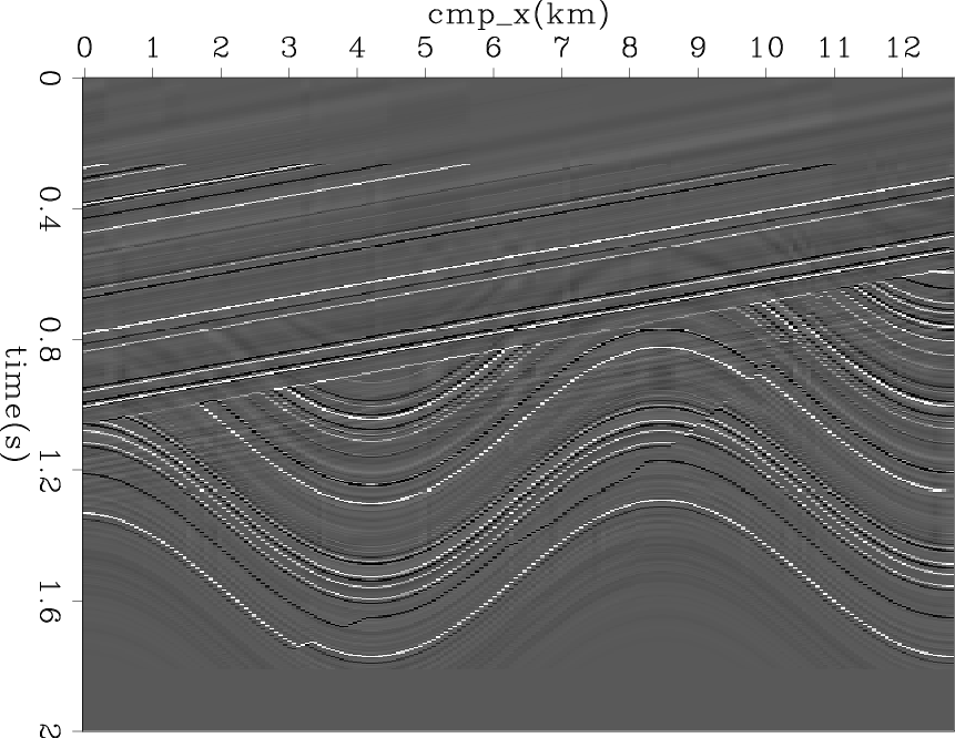
Figures 6(a) and 6(b) show the bidirectional deconvolution proposed by Shen et al. (2011) without and with PEF preconditioning. The deconvolution model with PEF preconditioning is more spiky than the one without preconditioning, but it still retains some slight ringing around the events. Recall that results in the 1D example show similar properties,, because the same wavelet is used to generate the data in the two examples.

mod3new,mod3newpre
Figure 6. Given the 2D synthetic data in Figure 5(b), (a) reflectivity model retrieved without preconditioning; (b) reflectivity model retrieved with PEF preconditioning.

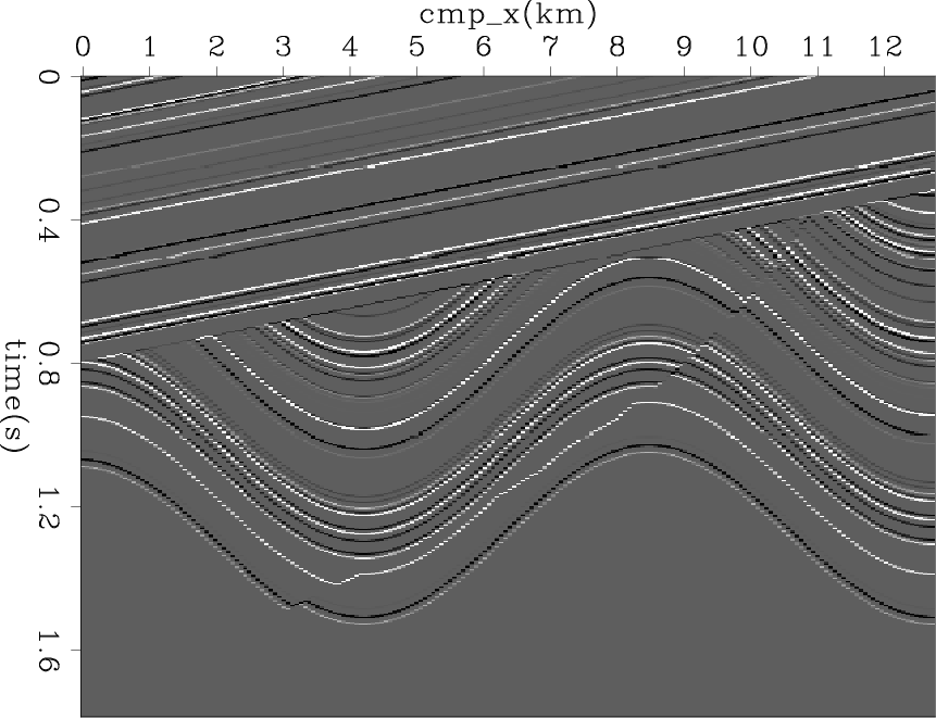
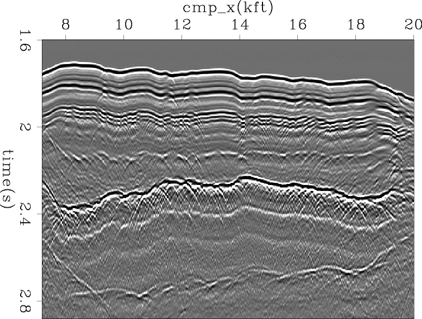
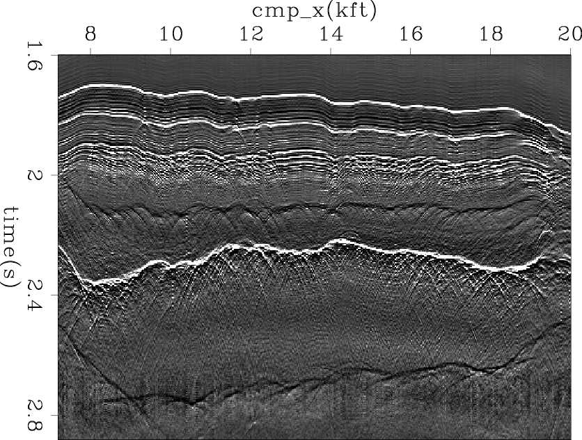
The last example is a common-offest section of marine field data. Figure 7 shows the input data. Figures 8(a) and 8(b) show the bidirectional deconvolution proposed by Shen et al. (2011) without and with PEF preconditioning. Both methods perform well to retrieve the sparse reflectivity in this field data. However, the preconditioned result has fewer precursors and cleaner events than the one without preconditioning. Another important difference is that around 2.4 seconds, there is an unknown event appearing in Figure 8(a), but it disappears in Figure 8(b). Thus we get a cleaner salt body when we apply preconditioning to this set of field data. The cause of the unknown event is still unidentified, but we have one possible explanation for this event. In this dataset, every trace looks identical, but with a time shift. There are two parallel events between 1.7 sec and 1.8 sec which have almost the same distance for all common midpoints. This phenomenon is unusual and may cause the unknown event, because the distance between the salt top and the unknown event is the same as that between the two parallel events. We hope the unknown event will disappear if we use another data set with more variable traces.

data4
Figure 7. Input Common Offset data.

mod4new,mod4newpre
Figure 8. Given the common offset data in Figure 7, (a) reflectivity model retrieved without preconditioning; (b) reflectivity model retrieved with PEF preconditioning.

Figures 9(a) and 9(b) show the shot wavelet estimated without and with PEF preconditioning. We notice that both results estimate the bubbles and the double ghost, which can be seen in the data. However, the estimated wavelet with preconditioning is more symmetric than the one without preconditioning. This symmetric quality meets our expectation that the wavelet we invert should look like a Ricker wavelet.

wavelet4new,wavelet4newpre
Figure 9. Given the common offset data in Figure 7, (a) shot wavelet estimated without preconditioning; (b) shot wavelet estimated with PEF preconditioning.

Preconditioning a non-linear problem and its application to bidirectional deconvolution