|
 |
 |
 | Fast automatic wave-equation migration velocity analysis using encoded simultaneous sources |  |
![[pdf]](icons/pdf.png) |
Next: numerical examples
Up: Tang: Encoded simultaneous-source WEMVA
Previous: introduction
I pose the velocity estimation problem as an optimization problem that tries to maximize
the image stack power across the reflection angle, taking advantage of the fact that
seismic events should be aligned and hence most constructively stacked in the angle domain,
if migrated using an accurate velocity model (Soubaras and Gratacos, 2007).
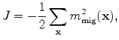
Instead of solving it as a maximization problem, I actually solve it as a minimization problem
that minimizes the negative image stack power. Because the reflection-angle stacked section is
equivalent to the zero-subsurface offset image, the objective function that I use to minimize
is therefore defined as follows:
 |
|
|
(1) |
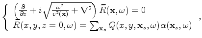
where
 is the zero-subsurface-offset image at image point
 , obtained by
crosscorrelating the forward propagated source wavefield with the backward propagated receiver wavefield
as follows:
, obtained by
crosscorrelating the forward propagated source wavefield with the backward propagated receiver wavefield
as follows:
 |
|
|
(2) |
where
 and
and
 are the source and receiver wavefield at image
point
are the source and receiver wavefield at image
point  , respectively,
for a source located at
, respectively,
for a source located at
 and at angular frequency
 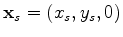 .
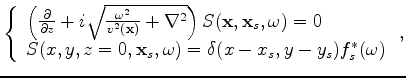
If a one-way extrapolator is used,
.
If a one-way extrapolator is used,  and
and  satisfy the following
one-way wave equations:
satisfy the following
one-way wave equations:
 |
|
|
(3) |
and
 |
|
|
(4) |
where 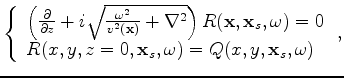 denotes taking the adjoint;
 is the velocity at image point
;
is the velocity at image point
;
 is the source signature;
 is the Dirac delta function;
 is the Laplacian operator.
 is the observed data mapped onto the computation grid, which is defined as follows:
 |
|
|
(5) |
where
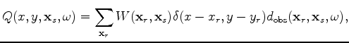 is the
observed data recorded at
is the
observed data recorded at
 due to a source at
  ;
;
 is the
acquisition mask operator, which contains ones where we record data and zeros where we do not.
is the
acquisition mask operator, which contains ones where we record data and zeros where we do not.
Since flat angle gathers generate the most coherent stack,
the negative image-stack-power minimization objective function defined by equation 1
is intuitive to understand. Objective function 1, however, has an alternative interesting
interpretation as shown in Appendix A, which proves that under the least-squares assumption,
minimization of objective function 1
is equivalent to the data-domain Born wavefield inversion, which minimizes the differences between the modeled
and observed primary reflections.
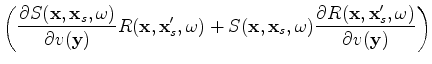
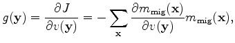
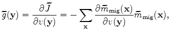
Objective function 1 is usually minimized using local optimization techniques, which require
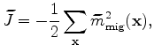
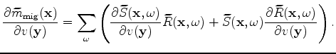
explicit calculation of the gradient. The gradient is obtained by
taking the derivative of  with respect to velocity
 (
( is the velocity coordinates) as follows:
 |
|
|
(6) |
where the sensitivity kernel, or tomographic operator,
 ,
can be easily obtained as follows:
,
can be easily obtained as follows:
 |
|
|
(7) |
Note the summations over
in equations 2 and 7.
This means that the computation for the image
 and the gradient
  needs to be carried out for each source independently,
resulting in a cost proportional to the number of sources.
The gradient
is usually calculated using the adjoint-state technique without explicitly constructing
the sensitivity kernel (Sava and Vlad, 2008; Shen, 2004; Tang et al., 2008).
needs to be carried out for each source independently,
resulting in a cost proportional to the number of sources.
The gradient
is usually calculated using the adjoint-state technique without explicitly constructing
the sensitivity kernel (Sava and Vlad, 2008; Shen, 2004; Tang et al., 2008).
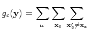
For encoded simultaneous-source WEMVA, the objective function to be minimized is defined as follows:
 |
|
|
(8) |
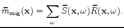
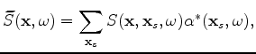
where the zero-subsurface-offset image
 is obtained by crosscorrelating the encoded source
wavefield,
is obtained by crosscorrelating the encoded source
wavefield,
 , and the encoded receiver wavefield,
 , as follows:
 |
|
|
(9) |
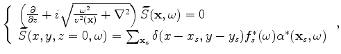
The encoded source and receiver wavefields satisfy the following one-way wave equations:
 |
|
|
(10) |
and
 |
|
|
(11) |
where
 is the phase encoding function. In this paper, I mainly focus on random phase encoding,
therefore
is the phase encoding function. In this paper, I mainly focus on random phase encoding,
therefore  is defined as follows:
 |
|
|
(12) |
where
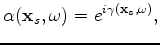 , and
, and
 is a uniformly distributed random sequence from 0
to
is a uniformly distributed random sequence from 0
to  .
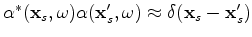
Tang (2011) shows that with this choice of random phase function,
has a zero expectation.
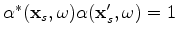
Note that the source encoding can be applied to data recorded from arbitrary types of acquisition geometries.
The simultaneous-source migrated image (
) will always converge to
the separate-source migrated image (
) as long as the encoding function satisfies
.
Tang (2011) shows that with this choice of random phase function,
has a zero expectation.
Note that the source encoding can be applied to data recorded from arbitrary types of acquisition geometries.
The simultaneous-source migrated image (
) will always converge to
the separate-source migrated image (
) as long as the encoding function satisfies
 .
.
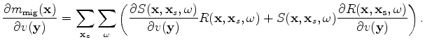
The gradient of objective function 8 is
 |
|
|
(13) |
where the tomographic operator,
 , in the encoded-source domain is defined as follows:
 |
|
|
(14) |
Note that equations 9 and 14 do not have a summation over the sources.
Therefore, the cost of computing the image
and the gradient
 is independent of the number of sources, as opposed to the separate-source case.
The gradient
is independent of the number of sources, as opposed to the separate-source case.
The gradient
 is also calculated using the adjoint-state technique using encoded simultaneous sources (Tang et al., 2008).
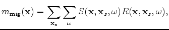
Although the computational cost of WEMVA is significantly reduced, encoded simultaneous sources add
crosstalk artifacts into the gradient. This becomes clear if we express
the encoded source and receiver wavefield as follows using the fact that wavefield propagation
is linear with respect to sources:
 |
|
|
(15) |
and
 |
|
|
(16) |
Substituting equations 15 and 16 into 14 and using
the fact that
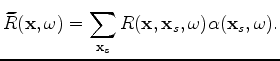 if
if
 yield
yield
 |
|
|
(17) |
where  is the crosstalk:
A way to mitigate the influence of crosstalk is to change the random encoding function at each iteration (Krebs et al., 2009),
so that the crosstalk will be destructively stacked over WEMVA iterations and consequently converge to zero
because it has a zero expectation. It is important to point out that regeneration of the random code
will result in the objective function (equation 8) changing at each iteration.
Therefore, the objective function may not be monotonically decreasing over iterations,
as opposed to the case in conventional separate-source WEMVA.
The optimization algorithm using encoded simultaneous sources is summarized in Algorithm 1.
|
|
|
|
| Fast automatic wave-equation migration velocity analysis using encoded simultaneous sources | |
|
Next: numerical examples
Up: Tang: Encoded simultaneous-source WEMVA
Previous: introduction
2011-09-13