Data examples of logarithm Fourier-domain bidirectional deconvolution

Preliminary Field data pre-stack shot gathers deconvolution result

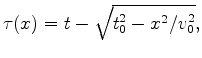
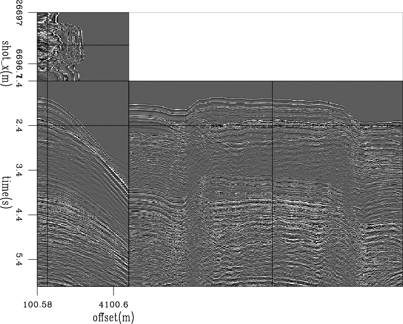
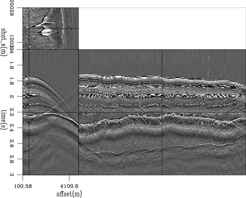
The common-offset data set we used in previous example section is extracted from a pre-stack survey line. Figure 7 shows the pre-stack shot gathers for the whole survey line. In order to see clearly the deep feature, we use a gain function of $t^{3}$ on figure 7. This gain function is only applied here for display purposes here and figure 8 shows two shot gathers in this survey without any gain applied. We also need gain function for deconvolution procedure to ensure the early time and late portion of data have the same weight to contribute to the solution. But We did not figure out what is a suitable gain function of this data set for deconvolution, so in the later test case, we use no gain function in deconvolution procedure.

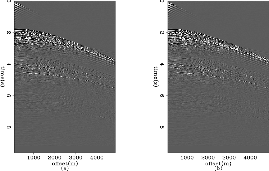
We find that the previous common-offset gather windowed the data not only in space but also in time. We want to get the data within the same time window as the previous common offset gather. But now we are working on the prestack gathers, and simply cutting a horizontal time window will lose the far-offset part of the deep event, due to the moveout. We do not preform a Normal Move Out correction (NMO) to correct the moveout, because we do not want the stretch caused by NMO to damage the shot waveform. Instead, we perform a constant time shift on each trace and try to flat one target event only. We use a major event in the desired time window, which is the reflection from the top of the salt body, as a target event to calculate the shift time. The shift time fucntion is

$$\tau(x)=t-\sqrt{t_0^2-x^2/v_0^2} ,$$ (9)

where $x$ is the offset, $v_0$ is a constant RMS velocity, $t$ is the travel time at $x$ offset of the target event and $t_0$ is the travel time at zero offset of the target event. The only unknow in equation 9 is $v_0$ . We can estimated $v_0$ by picking several points on the target event and do a regression. The Figure 9(a) shows the time-shift function to flatten the shot gather. We apply this time shift and then window the data set by time window 1.6 s to 3 s, figures 9(b) and (c) show two gathers after this window.

pre-cube
Figure 7. Whole marine pre-stack survey line.

2-gathers
Figure 8. Two shot gathers.

shifted-2-gathers
Figure 9. (a)The time shift function to flatten the gather; (b) and (c) two shifted shot gathers.

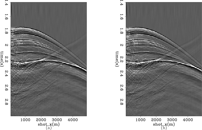
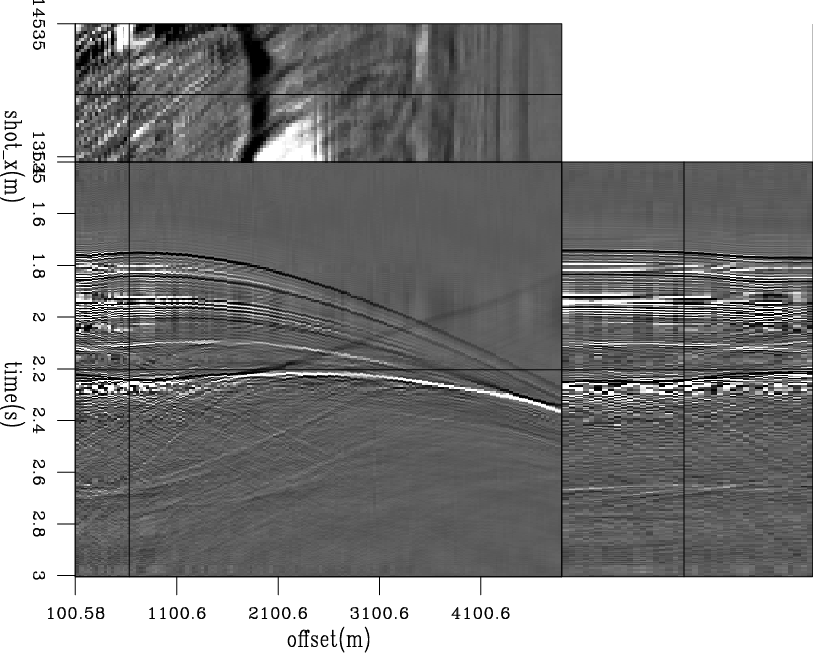
After we get the two windowed shot gathers, we apply the Burg PEF as the preconditioner and then perform the logarithm Fourier-domain bidirectional deconvolution on the two windowed shot gathers. Figure 10 shows the preconditioner results, and figure 11 shows the deconvolution results for the two shot gathers. The two shot gathers are processed independently, which means we use different Burg PEFs and different deconvolution filters on the two shot gathers.

shifted-2-decon
Figure 10. Two shot gathers after applying Burg PEF preconditioning. Different PEF filters are estimated and applied separately.

shifted-2-log-bidecon
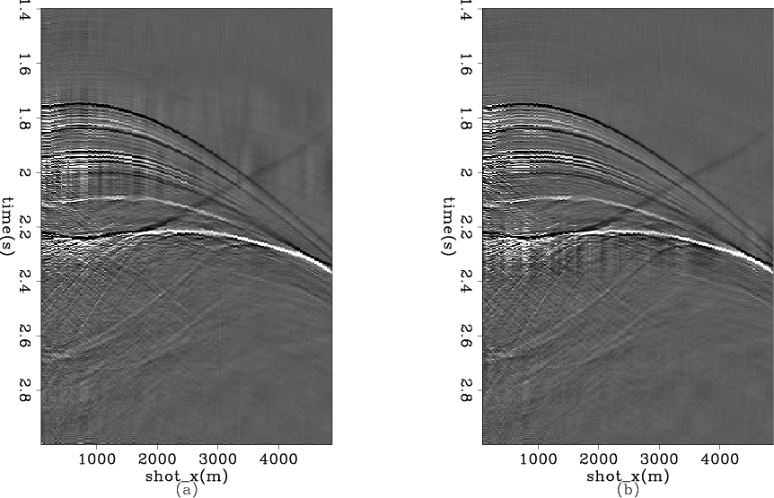
Figure 11. Two shot gathers after logarithm Fourier domain bidirectional deconvolution. The deconvolution is applied separately for each gather and within the same shot gather we use one costant deconvolution filter for all traces

The major event (in the vicinity of 2.2 s), which is the top of the salt body, has a phase shift with increasing offset. In figure 11, the near-offset part of this event is black, and then it turns white after an offset of about 1500 meters. The head wave starts at the same offset of 1500 meters. This is not coincidence, but occurs because the reflection has a $90^\circ$ phase shift after the critical angle.

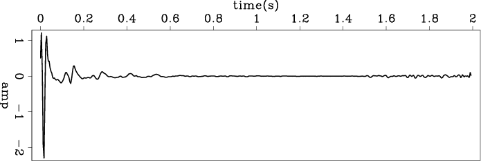
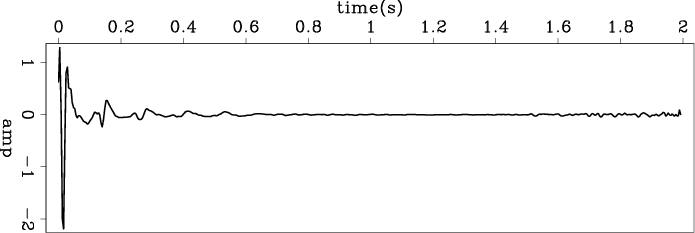
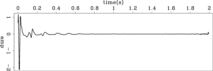
Figures 12(a) and 12(b) show the estimated wavelets of these two shot gathers. We see that these are quite similar, indicating that the shot waveforms do not change much between these two shots.

wavelet-shot-00,wavelet-shot-28
Figure 12. The estimated wavelets by logarithm Fourier-domain bidirectional deconvolution. (a) Shot gather 14000; (b) shot gather 14028. We notice that the in the Ricker part, (b) is less symmetric than (a), but we do not know exactly what cause this difference.

We also tried deconvolution of multi-shot gathers with one filter. Figures 13 and 14 show deconvolution results for 39 and 451 shot gathers, respectively, and figures 15(a), 15(b) and 15(c) show a comparison among estimated wavelets of single shot gathers and multi-shot gathers. The wavelets are similar, and from panels (a) to (c) we can see that using more shot gathers reduces jitter. These results tell us that the shot waveforms do not change significantly from shot to shot. This is consistent with our observations in the previous analysis of two shot gathers.

we notice in the figure 15(c), there is low frequency component which looks like a white stripe within the salt body. We do not have the similar thing in our common offset result (figure 4). We expect to get better deconvolution quality for pre-stack gathers due to we have more data, but the results show us the oppsite conclusion. That is a indicate the wavelet is various with offset changing. We need a way to use various wavelet for different offset range to handle this problem. But we can not simply divided the shot gathers into several vertical stripes because the wavelet is function of both offset and travel time (and maybe tavelling angle). We need more work to find out the pattern to separate shot gather into portions in which one portion has a relative constant wavelet. Furthermore, we also need to figure out the suitable gain function as the weighting for bidirectional deconvolution before we do more test on this pre-stack data set.

39-bidecon-cube
Figure 13. Logarithm Fourier-domain bidirectional deconvolution result on 39 shot gathers.

451-bidecon-cube
Figure 14. Logarithm Fourier-domain bidirectional deconvolution result on 451 shot gathers.

wavelet-1-shot,wavelet-39-shots,wavelet-451-shots
Figure 15. The wavelets estimated from (a) one shot gather (same as 12(a)); (b) 39 shot gathers (from shot location of 13500 meters to 14500 meters); (c) 451 shot gathers (from shot location of 8000 meters to 20000 meters).

Data examples of logarithm Fourier-domain bidirectional deconvolution