Elastic Born modeling in an ocean-bottom node acquisition scenario

Elastic Born forward modeling

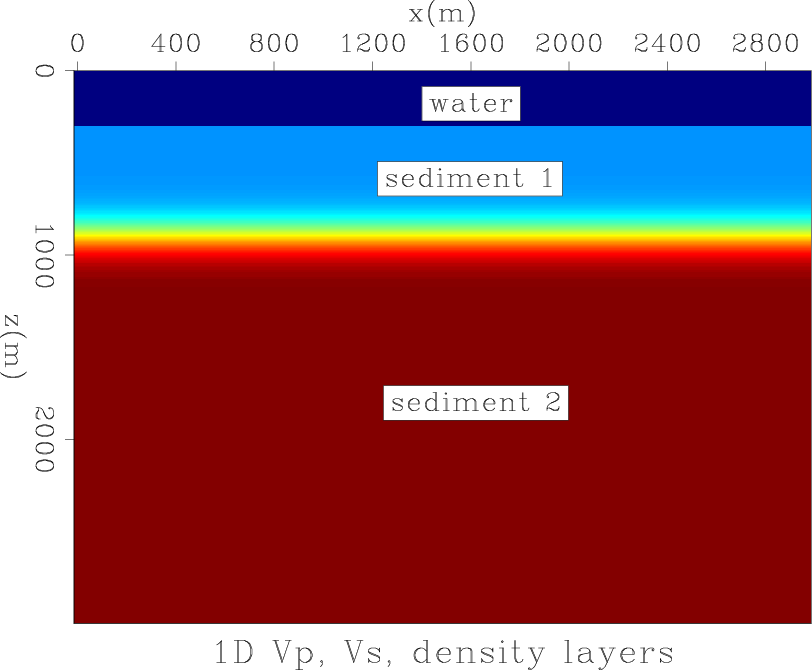
In the following examples, I used a 3 layer 1D model of acoustic velocity, shear velocity and density. The top layer was water, and there was a full spread of receivers located at the water bottom. Figure 3 represents the models used for the incident wavefield (sharp water bottom interface). In the models used to propagate the scattered wavefield, the layer marked ``sediment 1'' is extended all the way to the surface. The model parameters were:

$\rho_1 = 1025 \frac{kg}{m^3} \quad \quad \quad V_{p1} = 1500 \frac{m}{s} \quad \quad \quad V_{s1} = 0 \frac{m}{s}$
$\rho_2 = 1700 \frac{kg}{m^3} \quad \quad \quad V_{p2} = 1700 \frac{m}{s} \quad \quad \quad V_{s2} = 500 \frac{m}{s}$
$\rho_3 = 1600 \frac{kg}{m^3} \quad \quad \quad V_{p3} = 2200 \frac{m}{s} \quad \quad \quad V_{s3} = 1000 \frac{m}{s}$

smoothmods Figure 3. The smooth $\rho$ , $V_p$ and $V_s$ model representation for the incident wavefield.

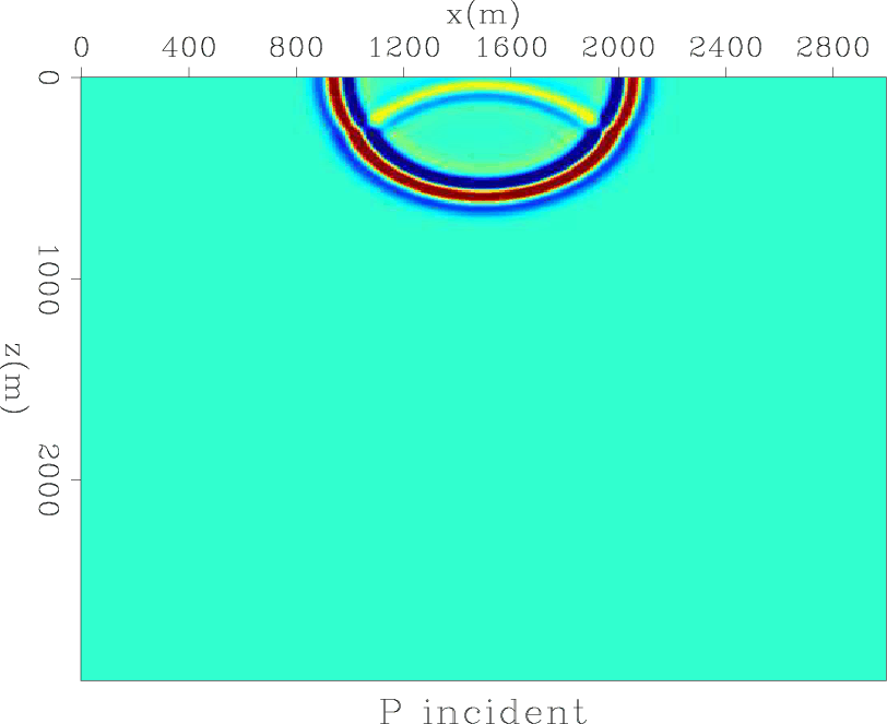
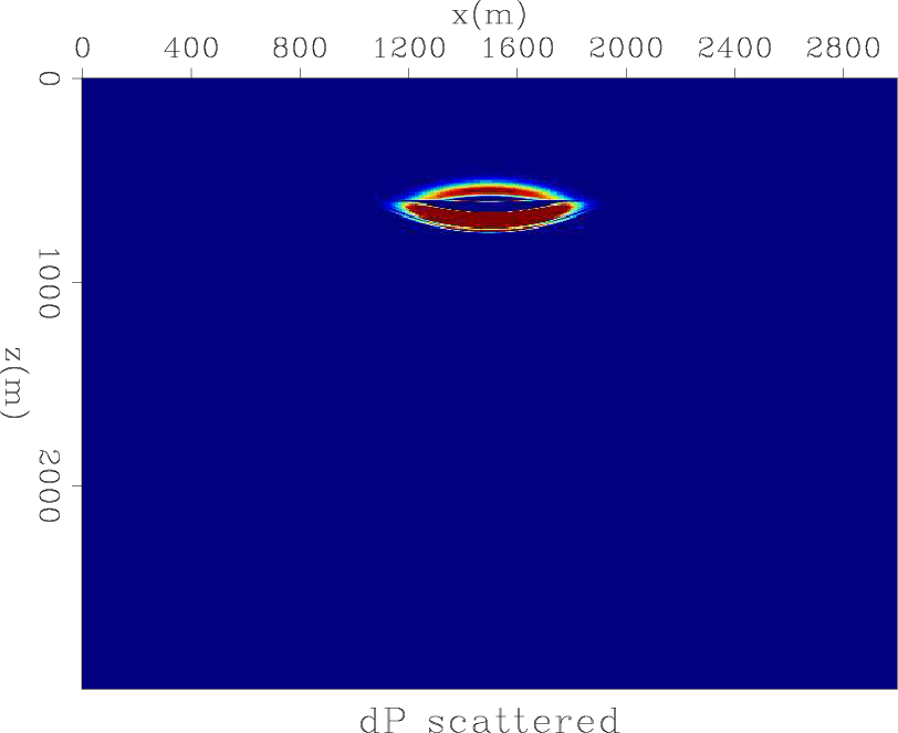
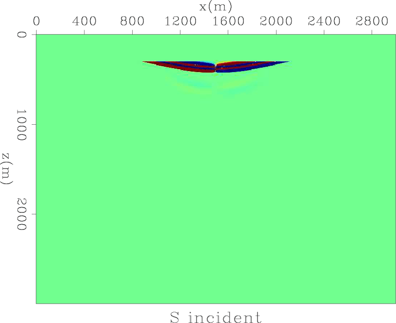
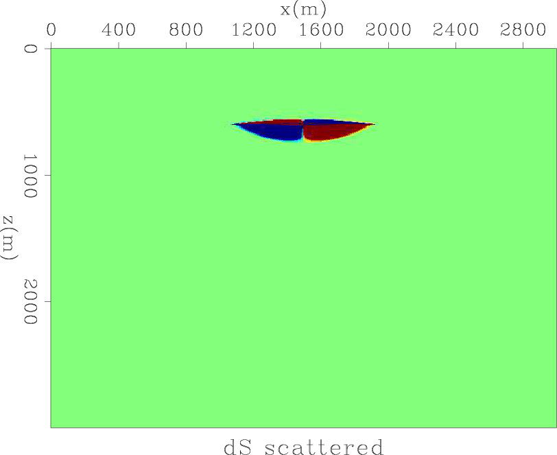
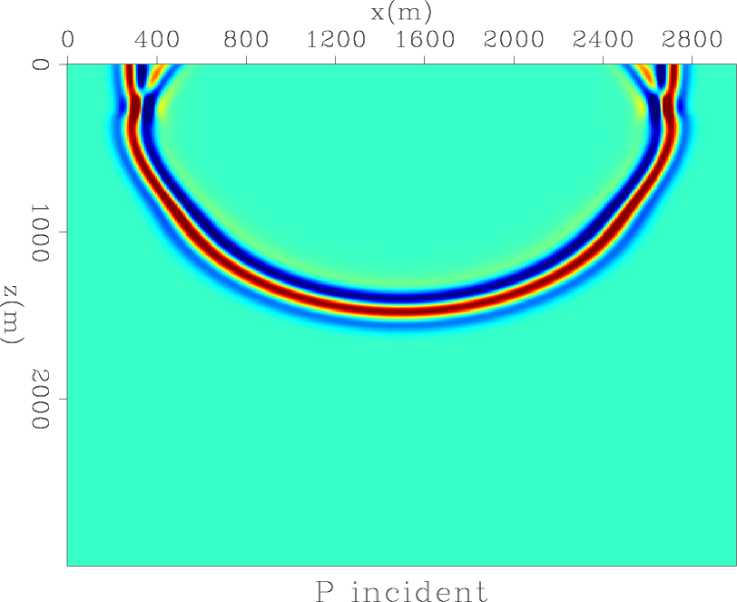
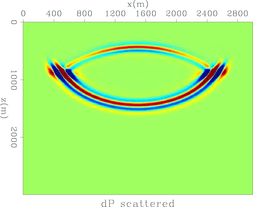
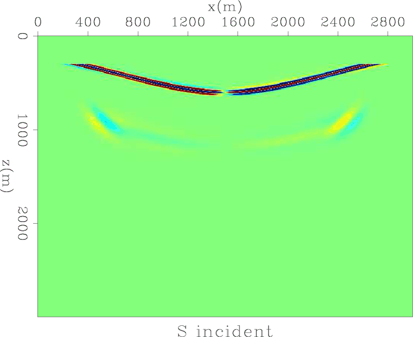
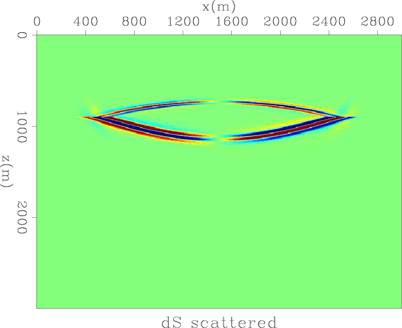
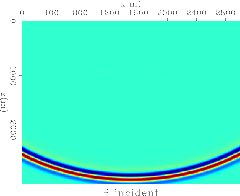
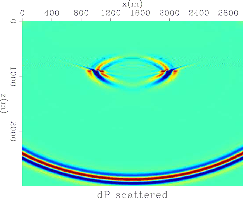
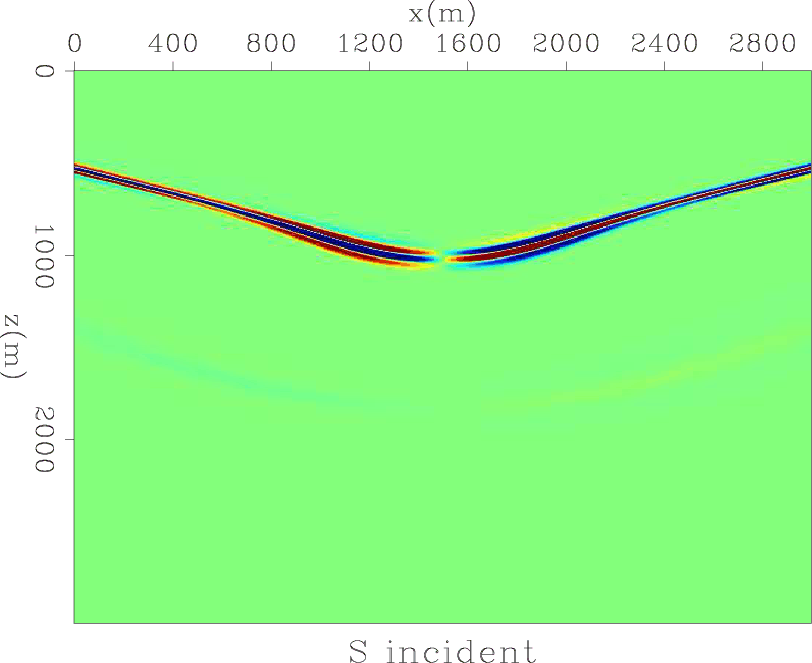
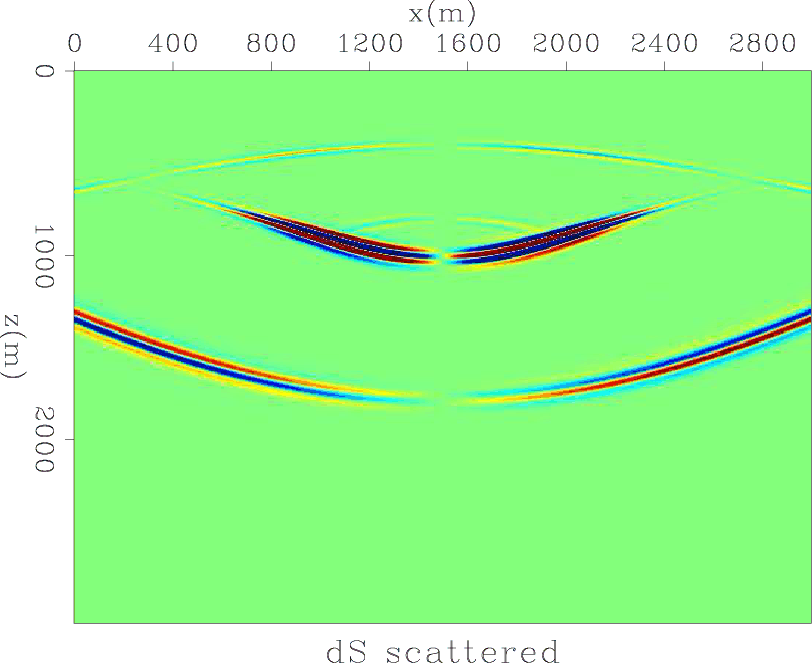
Figures 4(a)-4(l) show the incident and scattered P and S wavefields, which are a result of the application of equations 7 and 8 to the Born-modeled incident and scattered particle velocity fields. The rows are arranged by time snapshots, so at each row we see each field at the same time. The column order from left to right is incident P, scattered P, incident S, scattered S. In Figure 4(a) we can see the P reflection at the water bottom, resulting from the sharp boundary there. This reflection is absorbed by the attenuating boundaries. In Figure 4(b) and 4(f), the P reflection from the bottom reflector is visible. Figure 4(c) is the incident S-wave generated by mode conversion at the water-solid interface. Figures 4(d) and 4(h) show the scattered S-wave generated by a mode conversion at the bottom reflector. Figures 4(e) and 4(i) are the propagating incident P wavefield. In Figure 4(g), though it is the incident S field, we can still see a transmitted mode conversion from the incident P wavefield at the bottom reflector. In Figure 4(k), the S-wave has hit the bottom reflector, which is the reason that we see both a P and an S reflection in the scattered field in Figures 4(j) and 4(l).

0Psnap1,0dPsnap1,0Ssnap1,0dSsnap1,0Psnap2,0dPsnap2,0Ssnap2,0dSsnap2,0Psnap3,0dPsnap3,0Ssnap3,0dSsnap3
Figure 4. P and S incident and scattered wavefield snapshots at propagation times: t1=0.46s (top row), t2=0.9s (center row), t3=1.55s (bottom row).

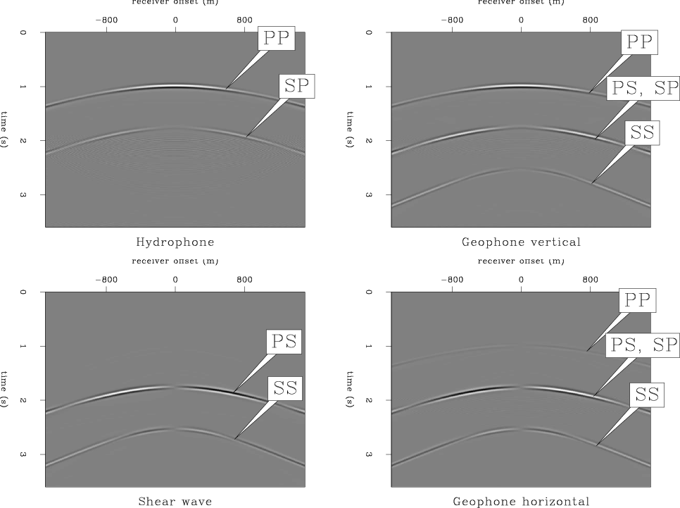
The simulation of OBN hydrophone recording is done by saving the scattered P wavefield one model cell above the sea bottom. The horizontal and vertical geophone recording is done by saving the vertical and horizontal particle velocity fields, within the solid layer at the sea bottom. The receivers are fully spread on the sea bottom. The source is an explosive source at the sea surface.

Figure 5 shows the recorded data components, generated by the elastic Born modeling. There is no direct arrival, since the water-solid interface is not used to generate scattering. Note that the shear wave recording is virtual. There is no recevier that records only shear waves. However, using equation 8 the shear wave value can be extracted from the particle-velocity fields at the sea bed. This information is useful for analyzing which of the reflections are P and which are S. The reflection types are pointed out in the figure. The label ``PP'' signifies a P-wave generated at the source position, which was transmitted at the water bottom as a P-wave, and was reflected as a P-wave at the bottom reflector within the sediment (Figure 3). The label ``PS'' signifies a similar path, except that at the bottom reflector a mode conversion occures, resulting in an upgoing S-wave. The label ``SP'' signifies a P-wave generated at the source position, which was converted at the sea bottom to a transmitted S-wave, and was converted again upon reflection at the bottom reflector to an upgoing P-wave.

Observing the hydrophone data and the virtual shear wave recording, we can see that the vertical and radial geophone components record both P and S-waves. Furthermore, we can see that the arrival at $t=1.8s$ contains two converted modes: PS and SP. They arrive at the same time, since the model is 1D. As a result of the single-scattering of the Born modeler, all data in Figure 5 are upgoing data, and therefore represent the result we expect to have from a perfect separation of the upgoing from the downgoing wavefields.

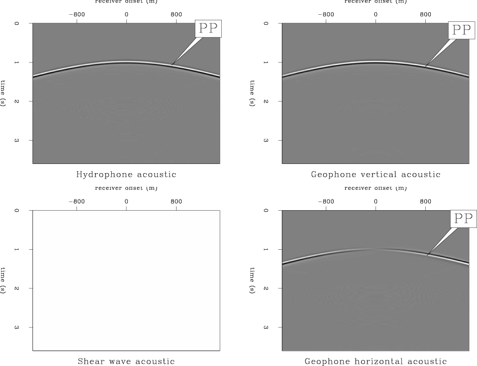
Figure 6 is the recording of data generated by acoustic Born modeling. In effect, I used the same code as for the elastic modeling, setting $V_s=0$ . This is the reason for the empty data in the virtual shear wave recording. As expected, there is only one PP arrival. Again - no direct wave is visible since the water-solid interface is not used to generate scattering. Like the previous elastic data example, this upgoing acoustic recording is what we expect from a perfect up/down separation.

0-recfigs-mute
Figure 5. Synthetic OBN data generated by elastic Born modeling. Top left: Hydrophone containing only P-wave data. Top right: Vertical geophone containing P and S-wave data. Bottom left: Shear wave virtual recording. Bottom right: Horizontal geophone containing P and S-wave data. Note the lack of a direct arrival, as a result of the water-solid interface not being used to generate scattering.

0-recfigs-mute-acous
Figure 6. Synthetic OBN data generated by acoustic Born modeling. Top left: Hydrophone containing only P-wave data. Top right: Vertical geophone containing only P-wave data. Bottom left: Shear wave virtual recording. Bottom right: Horizontal geophone containing only P data.

Elastic Born modeling in an ocean-bottom node acquisition scenario